Computer Solution of Goal Programming Problems with QM for Windows and Excel
| Goal programming problems can be solved using QM for Windows and Excel spreadsheets. In this section we will demonstrate how to use both computing alternatives to solve the Beaver Creek Pottery Company example we solved graphically in the previous section.
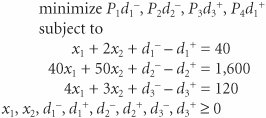
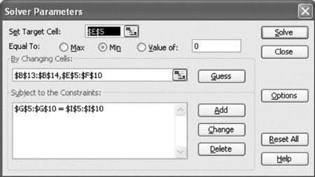
QM for WindowsWe will demonstrate how to solve a goal programming model by using our Beaver Creek Pottery Company example, which was formulated as follows : QM for Windows includes a goal programming module that can be accessed by clicking on the "Module" button at the top of the screen. The model parameters are entered onto the data input screen as shown in Exhibit 9.1. Notice that each prioritized deviational variable must be assigned a weight, which for this problem is always one. The solution is obtained by clicking on the "Solve" button at the top of the screen. The solution summary for our model is shown in Exhibit 9.2. Exhibit 9.1. Exhibit 9.2.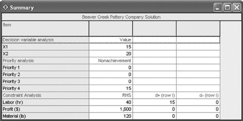 QM for Windows will also provide a graphical analysis of a goal programming model. We click on the "Windows" button and then select "Graph" from the menu. The graph for our example is shown in Exhibit 9.3. Exhibit 9.3.(This item is displayed on page 400 in the print version)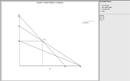 Excel SpreadsheetsSolving a goal programming problem by using Excel is similar to solving a linear programming model, although not quite as straightforward. Exhibit 9.4 shows the spreadsheet format for our Beaver Creek Pottery Company example. Cells G5, G6, and G7, under the heading "Constraint Total," contain the formulas for our goal constraints, including deviational variables. The formula for the labor constraint is shown on the formula bar at the top of the screen in Exhibit 9.4. The model decision variables are in cells B10 and B11, and the deviational variables are in cells E5:F7 . The goals are established by setting the constraint formulas in G5 to G7 equal to the goal levels in cells I5 to I7. Exhibit 9.4.(This item is displayed on page 400 in the print version)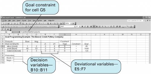 When using a spreadsheet (or any regular linear programming program) to solve a goal programming problem, it must be solved sequentially . In this procedure, a new problem is formulated and solved for each priority goal in the objective function, beginning with the highest priority. In other words, the minimization of the deviational variable at the highest priority is the initial objective. Once a solution for this formulation is achieved, the value of the deviational variable that is the objective is added to the model as a constraint, and the second-priority deviational variable becomes the new objective. A new solution is achieved for each new objective sequentially until all the priorities are exhausted or it is clear that a better solution cannot be reached. For our purposes, this means editing Excel's Solver for each new solution. Exhibit 9.5 shows the Solver Parameters window for our spreadsheet example. Recall that the first-priority goal for our model is the minimization of the negative deviational variable ( d 1 ) for our labor goal. This deviational variable is located in cell E5; thus, we start Solver by minimizing cell E5. We identify B10:B11 (the decision variables) as well as E5:F7 (the deviational variables) as variables in the model. The model constraints are for our goals (i.e., G5:G7 = I5:I7 ). Exhibit 9.5.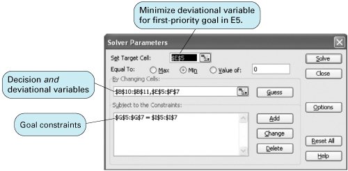 The spreadsheet with the solution to our example problem is shown in Exhibit 9.6. We know this is the most satisfactory solution we can achieve from the QM for Windows solution, so it will not be necessary to perform any additional sequential steps. From the spreadsheet we can see that we have achieved all the goals except the fourth-priority goal, to minimize d 1 + . However, if we had not achieved all our top goals so readily, the next step would be to include E5 = as a constraint in Solver and then minimize our next-priority goal, which would be E6 (i.e., d 2 ). Exhibit 9.6.(This item is displayed on page 401 in the print version)
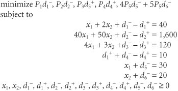
Next we will use Excel to solve a slightly more complicated goal programming modelthat is, the altered Beaver Creek Pottery Company example we developed at the beginning of this chapter, with goals for overtime and maximum storage levels for bowls and mugs: The spreadsheet for this modified version of our example is shown in Exhibit 9.7. The spreadsheet is set up much the same as the original version of this example, with the exception of the goal constraint for overtime. The formula for this goal constraint is included in cell G8 as = F5 + E8 F8 . In addition, the positive deviational variables for the last two goal constraints are now included in the formulas embedded in cells G9 and G10. For example, in cell G9 the constraint formula is = C9 * B13 + E9 . Exhibit 9.7.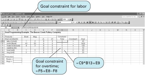 The Solver Parameters window for this spreadsheet is shown in Exhibit 9.8, and the resulting solution is shown in Exhibit 9.9. Exhibit 9.8.(This item is displayed on page 403 in the print version) Exhibit 9.9.(This item is displayed on page 403 in the print version)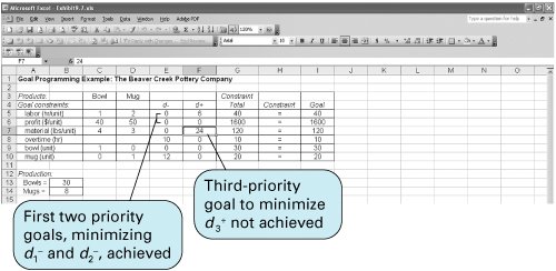 You will notice that this solution achieves the first two priority goals for minimizing d 1 and d 2 , which are in cells E5 and E6. However, the third-priority goal to minimize d 3 + is not achieved because its cell (F7) has a value of 24 in it. Thus, we must follow the sequential approach to attempt to obtain a better solution. We accomplish this by including E5=0 (the achievement of our first goal) as a constraint in Solver, as well as our second-priority goal that this solution achieved, E6=0 , and then minimizing F7. This Solver Parameters screen is shown in Exhibit 9.10. Exhibit 9.10.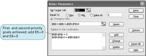 The solution is shown in Exhibit 9.11. This is the same solution that we obtained for our original version of the model, without the alterations for overtime and production levels. This solution achieves the first three priority goals. We could continue to attempt to achieve the fourth-priority goal by including F7 = 0 as a constraint in Solver and minimizing cell F5 (i.e., d 1 + ); however, doing so will not result in a better solution without sacrificing the goal achievement at the higher-priority levels. Thus, this is the best solution we can achieve. Exhibit 9.11.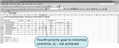 |
EAN: 2147483647
Pages: 358

