Section 10.2. Financial Functions | Excel 2007[c] The Missing Manual

10.2. Financial Functions

Excel includes several dozen financial formulas, but non- accountants use only a handful of these regularly. These all-purpose functions, described in the following sections, are remarkably flexible. You can use them to make projections about how investments or loans will change over time, or to answer hypothetical questions about investments or loans. Perhaps you want to determine the interest rate or length of time you need to reach an investment goal or pay off a loan.

10.2.1. FV( ): Future Value

The FV( ) function lets you calculate the future value of an investment, assuming a fixed interest rate. Perhaps the FV( ) function's most convenient feature is that it lets you factor in regular payments, which makes it perfect for calculating how money's accumulating in a retirement or savings account.

To understand how FV( ) works, it helps to start out by considering what life would be like without FV( ). Imagine that you've invested $10,000 that's earning a fixed interest rate of 5 percent over one year. You want to know how much your investment's going to be worth at the end of the year. You can tackle this problem quite easily with the following formula:

 =10000*105%

This calculation provides you with the future valuethat is, the initial 100 percent of the principal plus an additional 5 percent interest.

It's just as easy to determine what happens if you keep your money invested for two years , reinvesting the 5 percent interest payment for an additional year. Here's the formula for that:

 =10000*105%*105%

In the end, you wind up with a tidy $11,025.

Clearly, for these simple calculations, you don't need any help from Excel's financial functions. However, real accounts aren't always this simple. Here are two common problems that can make the aforementioned calculation a lot more difficult to solve when using a do-it-yourself formula:

You've invested your money in a savings account that pays interest monthly. Even though the annual rate of interest's the same as in the earlier examples, your money accumulates faster thanks to compound interest (that is, interest earned on the interest you've previously earned).
You make regular deposits to the investment account. You can't calculate this extra amount of money separately because it also accumulates interest, starting from the date on which you deposited it.

All of a sudden, this calculation isn't so easy to perform. Of course, you could solve it on your own, but the formula you'd need to write is startlingly complex. At this point, the FV( ) function becomes a lot more attractive. Here's how the function breaks down (remember, brackets indicate optional arguments):

 FV(rate, nper, payment, [pv], [type])

The rate is the interest rate your investment's earning.
The nper is the number of interest payments. If your account receives interest once a year and you invest your money over a two-year period, then the nper will be 2. If you're making regular contributions, this value also specifies the number of contributions you're making. FV( ) assumes that every contribution's made on the same day as the interest's generated, which is an unfortunate limitation. (You can get around this limitation by using FV( ) several times to calculate the value of individual contributions, and then adding these together.)
The payment is the amount of the contribution you want to make regularly. Set this to 0 if you don't want to add anything.
The pv is the present value, or the initial balance of your account. If you omit this value, then Excel assumes you start with nothing. As a result, you'll need to include something other than 0 for the payment.
The type indicates the timing of the payment. If you specify 0 (or omit this value), then the payment's made at the end of the period. If you specify 1, then the payment's made at the beginning, giving your interest just a little bit more time to compound.

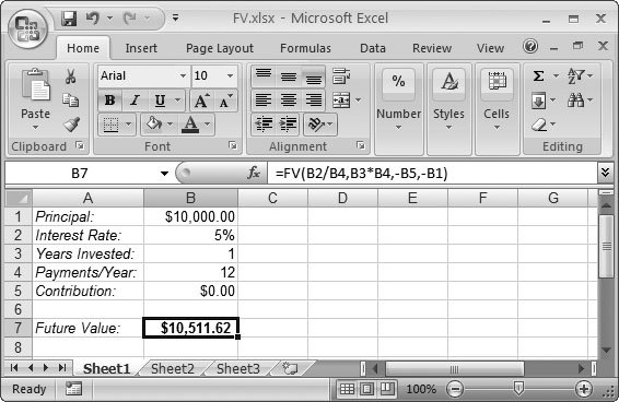
The only tricksome would say Bizarro World elementwith FV( ) is that you need to make sure both the payment and the initial balance (pv) are negative numbers (or zero values). Huh? Isn't this money that's accumulating for you? Here's what's going on: In Excel's thinking, the initial balance and the regular contributions are money you're handing over, so these numbers, consequently, need to be negative. The final value is positive because that's the total you're getting back.

Continuing with the earlier example, here's how you'd rewrite the formula that calculates the return on a $10,000 investment after one year earning 5 percent annual interest:

 =FV(5%, 1, 0, -10000)

Note: The formula knows that this is a one-year investment because the 5 percent is an annual interest rate, and you've indicated (through the second argument) that there's only one interest payment being made.

This calculation returns the expected value of $10,500. But what happens if you switch to an account that pays monthly interest? You now have 12 interest payment periods per year, and each one pays a twelfth of the total 5 percent interest (see Figure 10-1). Here's the revised formula:

 =FV(5%/12, 12, 0, -10000)

Note that two numbers are different from the original formula: the interest (divided by 12 because it's calculated per payment period) and the number of payment periods. The new total earned is a slightly improved $10,511.62.

Note: The interest rate and the number of payment periods must always use the same time scale. If payments are monthly, then you must use a monthly interest rate. (Remember, to calculate the monthly interest rate, just take the yearly interest rate and divide by 12.)

Figure 10-1. This worksheet depicts a future value calculation using the FV( ) function and the information in cells B1 to B5. In this example, the initial balance is $10,000, the interest is 5 percent (paid monthly), and you don't make any additional contributions. Note that the nper (number of interest payments) is calculated by multiplying Years Invested by Payments/Year.

Finally, here's the calculation over two years. The only number that changes is the number of payment periods.

 =FV(5%/12, 24, 0, -10000)

And while you're at it, why not check what happens if you make a monthly contribution of $100 to top up the fund? In this case, you'll make the payment at the beginning of the month. The required formula is shown here:

 =FV(5%/12, 24, -100, -10000, 1)

Now, the total tops $13,000 ($13,578.50 to be precise). Not bad for a little number crunching !

Incidentally, FV( ) works just as well on loan payments. Say you take out a $10,000 loan and decide to repay $200 monthly. Interest is set at 7 percent and calculated monthly. The formula that tells you your outstanding balancethat is, the amount that you still oweafter three years is as follows :

 =FV(7%/12, 3*12, -200, 10000)

Note that the balance begins positive, because it's money that you've received, while the payment's negative, because it's money you're paying out. After three years, you'll probably be disappointed to learn that the loan hasn't been paid off. The FV( ) function returns4,343.24, which is the balance remaining to be paid.

Note: The FV( ) function simply can't solve some of the more complex problems. It can't take into account, for example, payments that change, interest rates that change, or payments that aren't made on the same date as the interest date. You can sometimes deal with an interest rate that varies from one year to another by using the FV( ) function more than once, to calculate the years separately. Excel includes some more advanced functions that can help you outif you have an advanced accounting degree. If not, you may be interested in checking out a heavyweight reference book like Financial Analysis with Microsoft Excel, Fourth Edition, by Timothy Mayes and Todd Shank (South-Western College Pub, 2006).

FREQUENTLY ASKED QUESTION
Monthly Versus Annual Interest Rates

How do I compare monthly and annual interest rates ?

A dollar may always be a dollar, but a 5 percent interest rate may not always pay what you expect. The important factor is how often your interest's compounded, which all depends on how often the interest payments are paid to your account (or calculated against your loan). As you've seen with the FV( ) function examples (Section 10.2.1), if 5 percent interest is compounded monthly, then you have a chance to make a little extra cash. That's because your interest payments make it into your account before the year's over, giving you the chance to earn some additional interest on the amount of interest you've received so far.

When comparing different types of investments, it's often important to get a feeling for how much difference compound interest makes. Say you need to know which investment option is betterone that pays 5 percent after one year, or a savings account that pays a monthly interest of 4.75 percent. To answer this question, you can run the numbers with FV( ), or you can use a shortcut, available courtesy of the EFFECT( ) function. This financial function calculates the effective annual interest for an interest rate that's compounded multiple times. All you need to do is specify two arguments: the rate and the number of times it'll be compounded. In the case of a 4.75 percent rate compounded 12 times over the course of the year, here's your formula:

 =EFFECT(4.75%, 12)

This formula returns a result of 0.485, or 4.85 percent. In other words, 4.75 percent compounded monthly is equivalent to 4.85 percent compounded annually, provided you don't make any more payments during the lifetime of the investment. Assuming you don't need early access to your money, the 5 percent fixed investment's still the better deal. How much better? Well, once again, you could use FV( ) to calculate the future value. But seeing as you've used EFFECT( ) so far, why not just try the following shortcut?

 =(5%-EFFECT(4.75%,12)) * 10000

Keeping in mind Excel's precedence rules (Section 8.1.3), which specify that expressions inside parentheses get evaluated first, here's what's happening: first, the EFFECT( ) function repeats the calculation just performed, returning a value of 0.485. Excel then subtracts this value from 5 percent (0.5), leaving you with the difference between the two rates: about 0.15 percent. Once you multiply that by the total amount of money you've invested ($10,000), you'll get the extra bit of money you make.

In this example, the difference between the fixed investment and the savings account is a modest $14.52, which may be a price worth paying for flexibility.

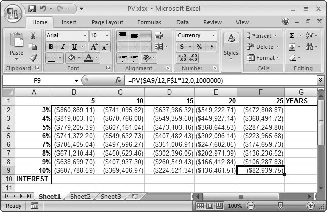
10.2.2. PV( ): Present Value

The PV( ) function calculates the initial value of an investment or a loan (which is also called the present value). The PV( ) function takes almost the same arguments as the FV( ) function, except the optional pv argument is replaced with an optional fv (or future value) argument:

 PV(rate, nper, payment, [fv], [type])

At first glance, the PV( ) function may not seem as useful as FV( ). Using future information to calculate a value from the past somehow seems counterintuitive. Can't people just dig up the principal value from their own records?

Yes, but the real purpose of PV( ) is to answer hypothetical questions. If you know what interest rate you can get for your money, how long you'll be invested, and what future value you hope to attain, you can pose the following question: What initial amount of money do I need to come up with? The PV( ) function can provide the answer.

Consider this formula:

 =PV(10%/12, 25*12, 0, 1000000)

The question Excel answers here is: In order to end up with $1,000,000, how much money do I need to invest initially, assuming a 10 percent annual interest rate (compounded monthly) and a maturation period of 25 years? The PV( ) function returns a modest result of $82,939.75.

If you don't have 25 years to wait, you can supplement your principal with a regular investment. The following formula assumes a monthly payment of $200, paid at the beginning of each month. Note that you should type in a negative number, because it's money you're giving up:

 =PV(10%/12, 25*12, -200, 1000000)

This change decreases the principal you need to a cool $60,930.30.

See Figure 10-2 for a much larger collection of PV formulas designed to answer the popular question: Who wants to be a millionaire? These formulas assume no monthly payment, and display the initial balance you need to reach a cool million. Sharp eyes will notice that the formula uses partially fixed references (like $A9 instead of A9). You can copy the formula from one cell to another without mangling the cell reference. $A9 tells Excel it can change the row but not the column. As a result, no matter where you copy it, this reference always points to the cell in column A of the current row (which holds the interest rate).

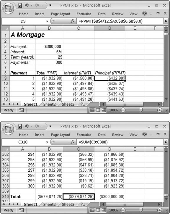
Figure 10-2. With the right amount of money and a sufficient amount of time, anyone can become a millionaire. This table shows the effect of different interest rates and investment time periods in an effort to make $1,000,000. The selected cell shows that if you assume your investment has 25 years to grow at 10% per year, you need to start out with $82,939.75 to hit the millionaire mark.

If you don't have the patience to wait for accruing money, you may be more interested in using PV( ) to determine how much money you can afford to borrow now . Assuming you can pay $250 a month for a three-year loan at a 7 percent annual interest rate, here's how you would calculate the size of the loan:

 =PV(7%/12, 3*12, -250, 0)

The answer? $8,096.62. In this example, the future value (fv) is 0 because you want to pay the loan off completely.

10.2.3. PMT( ), PPMT( ), and IPMT( ): Calculating the Number of Payments You Need to Make

The PMT( ) function calculates the amount of the regular payments you need to make, either to pay off a loan or to achieve a desired investment target. Its list of arguments closely resembles the FV( ) and PV( ) functions you've just learned about. You specify the present value and future value of the investment and the rate of interest over its lifetime, and the function returns the payment you'd need to make in each time period. Here's how the function breaks down:

 PMT(rate, nper, pv, [fv], [type])

If you don't specify a future value, then Excel assumes it's 0 (which is correct if you're performing the calculation to see how long it'll take to pay off a loan). Once again, the type argument indicates whether you make payments at the beginning of the payment period (1) or at the end (0).

To consider a few sample uses of the PMT( ) function, you simply need to rearrange the formulas you've been using in the FV( ) and PV( ) sections. If you have a 7 percent interest rate (compounded monthly) and a starting balance of $10,000, how much do you need to pay monthly to top it up to $1,000,000 in 30 years? The PMT( ) function provides your answer:

 =PMT(7%/12, 12*30, -10000, 1000000)

The result$753.16is a negative number because this is money that you're giving up each month.

A loan calculation is just as easy, although, in this case, the present value becomes positive, since it represents money you received when you took out the loan. To determine the payments needed to pay back a $10,000 loan (that comes with a 10 percent annual interest rate) over five years, you need this formula:

 =PMT(10%/12, 12*5, 10000, 0)

Assuming you make payments at the end of each month, the monthly payment is $212.47. If you add a type argument of 1 to pay at the beginning of the month, then this amount decreases to $210.71.

The PPMT( ) and IPMT( ) functions let you take a closer look at how you're repaying your loan, as they both analyze a single loan payment. PPMT( ) calculates the amount of a payment that's being used to pay down the loan's principal, while IPMT( ) calculates the amount of a payment that's being used to pay back accrued interest. You'll find both functions extremely useful if you need to figure, for tax purposes, what portion of your monthly loan payment's is paying interest, versus what portion's paying off a loan's principal (see Figure 10-3).

Figure 10-3. Top: A home mortgage is an ideal reason to use the PMT( ), PPMT( ), and IPMT( ) functions. This worksheet depicts each of the 300 mortgage payments you would make over the course of a 25-year $300,000 mortgage. The first payment contributes a measly $432.90 to paying off the principal.
Bottom: This table shows that the total of all payments made equals $579,871.26the amount you actually spent to pay off the $300,000 loan. This type of table is an amortization table.

Note: Over the course of a loan, the principal will gradually decrease, as will the amount of each payment going to pay the interest. But for each payment, it's always true that the PMT = PPMT + IPMT . In other words, your total monthly payment is always going to remain the same.

The PPMT() and IPMT( ) functions take the same arguments as the PMT( ) function with the only difference being that you need to specify one additional argument: per (short for period). This argument indicates which payment you're analyzing. For example, a per of 1 examines the first payment. A per of 6, meanwhile, analyzes the sixth payment, which, assuming you're paying the loan on a monthly basis, occurs halfway through the year. Here are both functions:

 PPMT(rate, per, nper, pv, [fv], [type]) IPMT(rate, per, nper, pv, [fv], [type])

As a quick example, consider the first payment of the $10,000 loan analyzed above using the PMT( ) function. You already know that each payment's $212.47. But what portion of this amount is actually paying down the principal? For the first payment, you can calculate the answer as follows:

 =PPMT(10%/12, 1, 12*5, 10000, 0, 0)

The answer's a relatively minute $129.14. On the last payment, however, the situation improves :

 =PPMT(10%/12, 12*5, 12*5, 10000, 0, 0)

Now a full $210.71 is used to pay off the last remaining bit of the balance.

Note: Clearly, the PPMT( ) and IPMT( ) functions don't work if you specify an argument of per that's greater than nper . In other words, you can't analyze a payment you don't make! Should you ever make this mistake, the function returns a #NUM! error value.

POWER USERS' CLINIC
Cumulative Interest and Principal Payments

The PPMT( ) and IPMT( ) functions let you analyze how much of a single payment pays a loan's principal, as well as the amount that pays interest. But what if you want to calculate the principal or interest payments over a range of payments? You can build an amortization table, like the one shown in Figure 10-3, or you can opt for a simpler choice: the CUMIPMT( ) and CUMPRINC( ) functions (which stand for cumulative interest payments and cumulative principal, respectively).

The CUMIPMT( ) function calculates the amount of money paid toward interest over a range of payments. Just specify the first and last payment you want to consider:

 CUMPIPMT(rate, nper, pv, first_per, last_per, type)

The following formula calculates the amount of interest paid over the first year (payments 1 to 12) of a $300,000 mortgage with a 25-year term .

 =CUMIPMT(6%/12, 25*12, 300000, 1, 12, 0)

The CUMPRINC( ) function performs a similar, but complimentary task. It has the same syntax, but instead calculates the amount of money paid toward the principal over a range of payments.

10.2.4. NPER( ): Figuring Out How Much Time You'll Need to Pay Off a Loan or Meet an Investment Target

The NPER( ) function calculates the amount of time it will take you to pay off a loan or meet an investment target, provided you already know the initial balance, the interest rate, and the amount you're prepared to contribute for each payment. Here's what the function looks like:

 NPER(rate, pmt, pv, [fv], [type])

If you're ready to contribute $150 a month into a savings account that pays 3.5 percent interest, you can use the following formula to determine how long it'll take to afford a new $4500 plasma television, assuming you start off with an initial balance of $500:

 =NPER(3.5%/12, -150, -500, 4500)

The answer is 25.48 payment periods. Remember, a payment period in this example is one month, so you need to save for over two years.

A similar calculation can tell you how long it'll take to pay off a line of credit. Assuming the line of credit's $10,000 at 6 percent, and you pay $500 monthly, here's the formula you would use:

 =NPER(6%/12, -500, 10000, 0)

In this case, the news isn't so good: It'll take 21 months before you're rid of your debt.

10.2.5. RATE( ): Figuring the Interest Rate You Need to Achieve Future Value

The RATE( ) function determines the interest rate you need to achieve a certain future value, given an initial balance, and a set value for regular contributions. The function looks like this:

 RATE(nper, pmt, pv, [fv], [type], [guess])

The math underlying the RATE( ) function's trickier than the calculations used in the other financial functions. In fact, there's no direct way to determine the interest rate if there's more than one payment made. Instead, Excel uses an iterative approach ( otherwise known as trial and error ). In most cases, Excel can quickly spot the answer, but if it comes up empty after 20 iterations, the formula fails and returns the dreaded #NUM! error code.

You can always supply an optional guess argument, which tells Excel what interest rate to try first. If you don't specify a rate, then Excel assumes 10 percent, and works from there. The guess must use the appropriate time scale, so if you're using monthly payments, remember to divide the yearly interest rate by 12. The number returned by the RATE( ) function also uses the same time scale.

Tip: It's all too easy to unintentionally ask an impossible question using the RATE( ) function. So make sure you're using realistic numbers when employing this function. Say you want to find out what interest rate you need to pay off a $10,000 loan in two years by making monthly payments of $225. If you attempt this calculation, then you'll get a negative value, indicating that there's no way to meet your goal unless the loan pays you interest.You could have avoided this mix up if you calculated the total amount of your monthly contributions ($225*24), which add up to only $5625.00. Clearly, this amount of money isn't enough to even pay off the $10,000 principal, let alone the interest!

Imagine you have a starting balance of $10,000. You make regular payments of $150, and you're hoping to double your money to $20,000 in three years. To determine the interest rate you need to make this a reality, use the following formula:

 =RATE(3*12, -150, -10000, 20000)

This calculation returns a monthly interest rate of 0.88 percent. You can generate the annual rate from this number by multiplying it by 12 (which gives you 10.5 percent, compounded monthly).

RATE( ) lends itself similarly well to loan calculations. Say you want to pay off a $5,000 loan in two years by making $225 payments each month. Here's the formula that determines the maximum annual rate you can afford.

 =RATE(2*12, -225, 5000, 0)*12

In this case, you need to find a loan that charges less than 7.5 percent annual interest.

10.2.6. NPV( ) and IRR( ): Net Present Value and Internal Rate of Return

NPV( ) is a more specialized function that can help you decide whether to make an investment or embark on a business venture by calculating net present value . To understand net present value, you first need to understand the concept of present value, which is the value that a projected investment has today . If you have an investment that earns 5 percent monthly interest and is worth $200 at maturity (after one month), its present value is $190.48.

You tackled present values with the PV( ) function described earlier in this chapter. The net present value's the same concept, except it applies to a series of cash flows (the profit, or loss, generated by an investment), rather than an investment with a fixed interest rate.

Practically speaking, people almost always use the NPV( ) function to compare the present value of an investment or business (sometimes called the venture investment ) to an investment with a fixed rate of return. The basic idea is simple: In order to be worthwhile, the venture investment must exceed a specific rate of return. If you know that you can get a 5 percent fixed rate of return from your bank, you won't consider using the money to open a coffee shop that's projected to make only 3 percent annually. (As always, Excel's financial functions take only cold, hard money into accountif opening a coffee shop is a lifelong dream, you may think differently.)

The NPV( ) function makes its calculation by examining cash flow over a series of years. You specify how much the venture investment cost you, or how much you received during each period, and NPV( ) calculates how that compares with an investment with a fixed rate. To conduct this comparison, you must choose an interest rate for the venture investment you're comparing against the fixed investment. This investment rate is called the discount rate . If the final NPV( ) value is negative, you'd have been better off with the fixed investment. If the NPV( ) value is positive, your venture is exceeding the fixed investment option.

Imagine you want to start a new coffee shop business. You're prepared to invest $25,000 to start off, and you expect to realize profits of $2,000 in the first year. In the following years, your profit projections are $6,500, $10,000, and $12,500. Simple addition tells you that this business will earn $31,000 in four years (and a net profit of $6,000). However, you also need to account for the interest you could receive by investing the cash profits at 5 percent as soon as they become available. Based on this scenario, how would your business (the venture investment) compare to a fixed security that earns 5 percent each year? You can answer that question using NPV( ).

The NPV( ) function (see Figure 10-4) requires the discount rate, and then a series of payments (or a cell range that contains a series of payments). Here's how to calculate the net present value of the four-year investment:

 =NPV(5%, 2000, 6500, 10000, 12500)

Excel counts each cash flow as one period. Thus, this formula goes through four periods. Because this formula uses an annual interest rate, each period represents a full year. The formula returns a result of $26,722.61. In other words, in order to generate the same amount of money as your business will, you'd need to invest $26,722.61 initially at an annual interest rate of 5 percent. This amount's more than the outlay required by our hypothetical business (which needs only $25,000 to get off the ground), so the business is a better place to put your money.

Or to put it another way, the present value of the business today is $26,722.61, even though you haven't ordered a sign or chosen a name . Because it costs only $25,000 to build the business, you'll be ahead of the game as soon as you set up shop (assuming, of course, you meet your profit projections).

Another way to look at net present values is to calculate the total money you've gained by subtracting the cost of your initial investment, as shown here:

 =NPV(5%, 2000, 6500, 10000, 12500) - 25000

In this case, as long as the result's greater than $0, it's a go. In this example, the difference is $1,722.61. The business is worth this much today, over and above the outlay required to get it started.

Note: In this example, the business made money each and every year. However, you could still use NPV( ) even if some years show a negative cash flow (although this won't help your rate of return).

TROUBLESHOOTING MOMENT
Subtle Problems with NPV( )

No one ever said that financial accounting is easy. In fact, the NPV( ) function is a good example of accounting's limitations, as it's littered with caveats that can easily trip you up.

For instance, you'll see that in order to calculate the real net present value, you need to subtract the initial investment cost after you use the function. You might wonder why you can't include a cost of $25,000 as one of the cash flows for NPV( ), like this:

 =NPV(5%, -25000, 2000, 6500, 10000, 12500)

This formula assumes that the $25,000 cost occurs after the first period, which is incorrect. Also, the NPV( ) function now assumes that five years have elapsed, instead of four, further skewing the answer. These problems occur because NPV( ) is sensitive to the time value of money. Time value is an expression economists use to emphasize the fact that $95 dollars today isn't worth the same as $95 in one yearbecause the earlier you get the money, the more time you have to earn interest. Adding arguments or changing their order can cause a different result.

Another problem with NPV( ) is that it assumes you're able to reinvest your business's earnings at a rate comparable to the set interest rate you're using to calculate NPV (in this case, 5 percent). However, if you're unable to invest the profit at 5 percent (perhaps because you need a shorter term investment that earns less), then you're not generating as much profit as the NPV( ) function indicates.

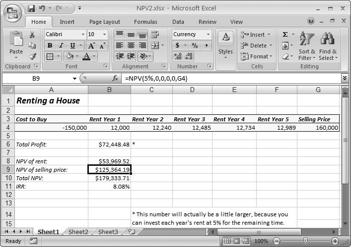
The NPV( ) function is particularly useful for evaluating prospective real estate investments. Consider what happens if you buy a condominium , rent it out for several years, and then sell it for the original price. If you take the rent money you earn (or predict you're going to earn), the NPV( ) function can tell you whether you'd be better off investing your money at a fixed interest rate. Figure 10-4 shows an example.

In Figure 10-4, NPV( ) suggests that the rent you stand to earn (a total of $62,448. 48, calculated by summing the rent collected in each year) is worth about $53,569 today. But you need to factor in the price of the property, which may increase or decrease. In this case, the property's estimated selling price ($160,000, which represents a measly gain of $10,000) makes it equivalent to having $125,364.19 to invest today at 5 percent interest. Thus, you're losing money on the value of the property (versus the rate of return you could get in the bank), but the rent you're earning more than makes up for it. By adding these two factors (property value and rent), you get a total net present value of $179,333.71. And because you purchased the property with only $150,000, this is very good news. If you still have doubts , look at the internal rate of return in cell B11 (the IRR( ) function is explained in Section 10.3). It shows that you're earning the equivalent of 8.08 percentsignificantly more than 5 percentfrom your real estate dealings.

Figure 10-4. This worksheet helps figure out whether it makes more sense to invest $150,000 at a fixed rate, or to use that money to buy and rent out a property.

The IRR( ) function is closely related to NPV( ). The main difference is that while NPV( ) calculates the value of the business or investment today, IRR( ) calculates how fast the business or rate appreciates in value (its rate of return). Technically, IRR( ) calculates the internal rate of return, which is the effective return rate based on your cash flows. In order to make this calculation, you must include the initial investment number with the cash flow. In fact, you need to supply all the values as a range, like so:

 =IRR(A4:G4)

This calculation returns 7.35 percent for the coffee shop business introduced in Section 10.2.6, and 8.08 percent in the rental property scenario illustrated in Figure 10-4.

Warning: The IRR( ) function is dangerous! While the NPV( ) function assumes you can reinvest your money at the rate you've specified (in the first argument), the IRR( ) function assumes that you can reinvest your money in the business for the same rate of return, which often isn't possible. Both NPV( ) and IRR( ) calculations are just estimates, and you need to carefully evaluate them.