Getting Started

Spatial Prediction Using Kriging, Contour Plots

After an appropriate variogram model is chosen , there are a number of choices involved in producing the kriging surface. In order to illustrate these choices, the variogram model in the the section Getting Started on page 4852 section of Chapter 80, The VARIOGRAM Procedure, is used. This model is Gaussian,

with a scale of c = 7 . 5 and a range of a = 30.

The first choice is whether to use local or global kriging. Local kriging uses only data points in the neighborhood of a grid point; global kriging uses all data points.

The most important consideration in this decision is the spatial covariance structure. Global kriging is appropriate when the correlation range ˆˆ is approximately equal to the length of the spatial domain. The correlation range ˆˆ is the distance r _ˆˆ at which the covariance is 5% of its value at zero. That is,

For a Gaussian model, r _ˆˆ is (thousand ft). The data points are scattered uniformly throughout a 100 — 100 (10 ⁶ ft ² ) area. Hence, the linear dimension of the data is nearly double the ˆˆ range. This indicates that local kriging rather than global kriging is appropriate.

Local kriging is performed by using only data points within a specified radius of each grid point. In this example, a radius of 60 (thousand ft) is used. Other choices involved in local kriging are the minimum and maximum number of data points in each neighborhood (around a grid point). The minimum number is left at the default value of 20; the maximum number defaults to all observations in the data set.

The last step in contouring the data is to decide on the grid point locations. A convenient area that encompasses all the data points is a square of length 100 (thousand ft). The spacing of the grid points depends on the use of the contouring; a spacing of five distance units (thousand ft) is chosen for plotting purposes.

The following SAS code inputs the data and computes the kriged surface using these parameter and grid choices. The kriged surface is plotted in Figure 37.1, and the associated standard errors are plotted in Figure 37.2. The standard errors are smaller where more data are available.

  data thick;   input east north thick @@;   datalines;   0.7  59.6  34.1   2.1  82.7  42.2   4.7  75.1  39.5   4.8  52.8  34.3   5.9  67.1  37.0   6.0  35.7  35.9   6.4  33.7  36.4   7.0  46.7  34.6   8.2  40.1  35.4   13.3   0.6  44.7  13.3  68.2  37.8  13.4  31.3  37.8   17.8   6.9  43.9  20.1  66.3  37.7  22.7  87.6  42.8   23.0  93.9  43.6  24.3  73.0  39.3  24.8  15.1  42.3   24.8  26.3  39.7  26.4  58.0  36.9  26.9  65.0  37.8   27.7  83.3  41.8  27.9  90.8  43.3  29.1  47.9  36.7   29.5  89.4  43.0  30.1   6.1  43.6  30.8  12.1  42.8   32.7  40.2  37.5  34.8   8.1  43.3  35.3  32.0  38.8   37.0  70.3  39.2  38.2  77.9  40.7  38.9  23.3  40.5   39.4  82.5  41.4  43.0   4.7  43.3  43.7   7.6  43.1   46.4  84.1  41.5  46.7  10.6  42.6  49.9  22.1  40.7   51.0  88.8  42.0  52.8  68.9  39.3  52.9  32.7  39.2   55.5  92.9  42.2  56.0   1.6  42.7  60.6  75.2  40.1   62.1  26.6  40.1  63.0  12.7  41.8  69.0  75.6  40.1   70.5  83.7  40.9  70.9  11.0  41.7  71.5  29.5  39.8   78.1  45.5  38.7  78.2   9.1  41.7  78.4  20.0  40.8   80.5  55.9  38.7  81.1  51.0  38.6  83.8   7.9  41.6   84.5  11.0  41.5  85.2  67.3  39.4  85.5  73.0  39.8   86.7  70.4  39.6  87.2  55.7  38.8  88.1   0.0  41.6   88.4  12.1  41.3  88.4  99.6  41.2  88.8  82.9  40.5   88.9   6.2  41.5  90.6   7.0  41.5  90.7  49.6  38.9   91.5  55.4  39.0  92.9  46.8  39.1  93.4  70.9  39.7   94.8  71.5  39.7  96.2  84.3  40.3  98.2  58.2  39.5   ;   proc krige2d data=thick outest=est;   pred var=thick r=60;   model scale=7.5 range=30 form=gauss;   coord xc=east yc=north;   grid x=0 to 100 by 5 y=0 to 100 by 5;   run;   proc g3d data=est;   title 'Surface Plot of Kriged Coal Seam Thickness';   scatter gyc*gxc=estimate / grid;   label gyc      = 'North'   gxc      = 'East'   estimate = 'Thickness'   ;   run;   proc g3d data=est;   title 'Surface Plot of Standard Errors of Kriging Estimates';   scatter gyc*gxc=stderr / grid;   label gyc    = 'North'   gxc    = 'East'   stderr = 'Std Error'   ;   run;  

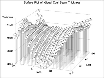
Figure 37.1: Surface Plot of Kriged Coal Seam Thickness

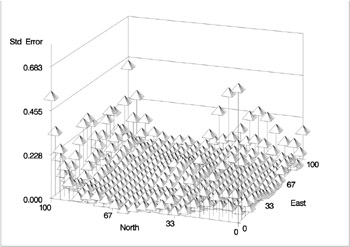
Figure 37.2: Surface Plot of Standard Errors of Kriging Estimates