Automatic Smoothing Parameter Selection
There are several methodologies for automatic smoothing parameter selection. One class of methods chooses the smoothing parameter value to minimize a criterion that incorporates both the tightness of the fit and model complexity. Such a criterion can usually be written as a function of the error mean square, ![]() 2 , and a penalty function designed to decrease with increasing smoothness of the fit. This penalty function is usually defined in terms of the matrix L such that
2 , and a penalty function designed to decrease with increasing smoothness of the fit. This penalty function is usually defined in terms of the matrix L such that
where y is the vector of observed values and · is the corresponding vector of predicted values of the dependent variable. Examples of specific criteria are generalized cross-validation (Craven and Wahba 1979) and the Akaike information criterion (Akaike 1973). These classical selectors have two undesirable properties when used with local polynomial and kernel estimators: they tend to undersmooth and tend to be non-robust in the sense that small variations of the input data can change the choice of smoothing parameter value significantly. Hurvich, Simonoff, and Tsai (1998) obtained several bias-corrected AIC criteria that limit these unfavorable properties and perform comparably with the plug-in selectors (Ruppert, Sheather, and Wand 1995). PROC LOESS provides automatic smoothing parameter selection using two of these bias-corrected AIC criteria, named AIC C 1 and AIC C in Hurvich, Simonoff, and Tsai (1998), and generalized cross-validation, denoted by the acronym GCV.
The relevant formulae are
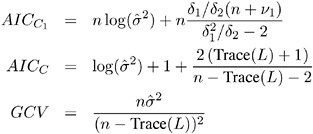
where n is the number of observations and
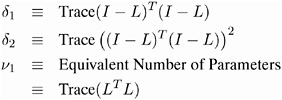
Note that the values of 1 , 2 , and the Equivalent Number of Parameters are reported in the Fit Summary table.
You invoke these methods for automatic smoothing parameter selection by specifying the SELECT= criterion option in the MODEL statement, where criterion is one of AICC1, AICC, or GCV. PROC LOESS evaluates the specified criterion for a sequence of smoothing parameter values and selects the value in this sequence that minimizes the specified criterion. If multiple values yield the optimum, then the largest of these values is selected.
A second class of methods seeks to set an approximate measure of model degrees of freedom to a specified target value. These methods are useful for making meaningful comparisons between loess fits and other nonparametric and parametric fits. The approximate model degrees of freedom in a nonparametric fit is a number that is analogous to the number of free parameters in a parametric model. There are three commonly used measures of model degrees of freedom in nonparametric models. These criteria are Trace( L ), Trace( L T L ), and 2Trace L ˆ’ Trace( L T L ). A discussion of their properties can be found in Hastie and Tibshirani (1990). You invoke these methods by specifying the SELECT= DFCriterion ( target ) option in the MODEL statement, where DFCriterion is one of DF1, DF2, or DF3. The criterion that is minimized is given in the following table:
| Syntax | Minimization Criterion |
|---|---|
| SELECT=DF1( target ) | Trace( L ) ˆ’ target |
| SELECT=DF2( target ) | Trace( L T L ) ˆ’ target |
| SELECT=DF3( target ) | 2Trace( L ) ˆ’ Trace( L T L ) ˆ’ target |
The results are summarized in the Smoothing Criterion table. This table is displayed whenever automatic smoothing parameter selection is performed. You can obtain details of the sequence of models examined by specifying the DETAILS(MODELSUMMARY) option in the model statement to display the Model Summary table.
There are several ways in which you can control the sequence of models examined by PROC LOESS. If you specify the SMOOTH= value-list option in the MODEL statement, then only the values in this list are examined in performing the selection. For example, the following statements select the model that minimizes the AICC1 criterion among the three models with smoothing parameter values 0 . 1, 0 . 3,and0 . 4:
proc loess data=notReal; model y= x1/ smooth=0.1 0.3 0.4 select=AICC1; run;
If you do not specify the SMOOTH= option in the model statement, then by default PROC LOESS uses a golden section search method to find a local minimum of the specified criterion in the range (0 , 1]. You can use the RANGE( lower , upper ) modifier in the SELECT= option to change the interval in which the golden section search is performed. For example, the following statements request a golden section search to find a local minimizer of the GCV criterion for smoothing parameter values in the interval [0.1,0.5]:
proc loess data=notReal; model y= x1/select=GCV( range(0.1,0.5) ); run;
If you want to be sure of obtaining a global minimum in the range of smoothing parameter values examined, you can specify the GLOBAL modifier in the SELECT= option. For example, the following statements request that a global minimizer of the AICC criterion be obtained for smoothing parameter values in the interval [0 . 2 , . 8]:
proc loess data=notReal; model y= x1/select=AICC( global range(0.2,0.8) ); run;
Note that even though the smoothing parameter is a continuous variable, a given range of smoothing parameter values corresponds to a finite set of local models. For example, for a data set with 100 observations, the range [0 . 2 , . 4] corresponds to models with 20 , 21 , 22 , , 40 points in the local neighborhoods. If the GLOBAL modifier is specified, all possible models in the range are evaluated sequentially.
Note that by default PROC LOESS displays a Fit Summary and other optionally requested tables only for the selected model. You can request that these tables be displayed for all models in the selection process by adding the STEPS modifier in the SELECT= option. Also note that by default scoring requested with SCORE statements is done only for the selected model. However, if you specify the STEPS in both the MODEL and SCORE statements, then all models evaluated in the selection process are scored.
In terms of computation, AIC C , GCV , and DF1 depend on the smoothing matrix L only through its trace. In the direct method, this trace can be computed efficiently . In the interpolated method using kd trees, there is some additional computational cost but the overall work is not significant compared to the rest of the computation. In contrast, the quantities 1 , 2 , and ½ 1 , which appear in the AIC C 1 criterion, and the DF2 and DF3 criteria, depend on the entire L matrix and for this reason, the time needed to compute these quantities dominates the time required for the model fitting. Hence SELECT=AICC1, SELECT=DF2, and SELECT=DF3 are much more computationally expensive than SELECT=AICC, SELECT=GCV, and SELECT=DF1, especially when combined with the GLOBAL modifier. Hurvich, Simonoff, and Tsai (1998) note that AIC C can be regarded as an approximation of AIC C 1 and that the AIC C selector generally performs well in all circumstances.
For models with one dependent variable, PROC LOESS uses SELECT=AICC as its default, if you specify neither the SMOOTH= nor SELECT= options in the MODEL statement. With two or more dependent variables, automatic smoothing parameter selection needs to be done separately for each dependent variable. For this reason automatic smoothing parameter selection is not available for models with multiple dependent variables . In such cases you should use a separate PROC LOESS step for each dependent variable, if you want to use automatic smoothing parameter selection.
Sparse and Approximate Degrees of Freedom Computation
As noted in the Statistical Inference section on page 2243, obtaining confidence limits in loess models requires the computation of the lookup degrees of freedom. This in turn requires the computation of
where L is the LOESS smoothing matrix (see the Automatic Smoothing Parameter Selection section on page 2243).
The work in a direct implementation of this formula grows as n 3 , where n is the number of observations in analysis. For large n , this work dominates the time needed to fit the loess model itself. To alleviate this computational bottleneck, Cleveland and Grosse (1991) and Cleveland, Grosse, and Shyu (1992) developed approximate methods for estimating this quantity in terms of more readily computable statistics. A different approach to obtaining a computationally cheap estimate of 2 has been implemented in PROC LOESS.
For large data sets with significant local structure, the LOESS model is often used with small values of the smoothing parameter. Recalling that the smoothing parameter defines the fraction of the data used in each local regression, this means that the loess fit at any point in regressor space depends on only a small fraction of the data. This is reflected in the smoothing matrix L whose ( i, j )th entry is nonzero only if the i th and j th observations lie in at least one common local neighborhood. Hence the smoothing matrix is a sparse matrix (has mostly zero entries) in such cases. By exploiting this sparsity PROC LOESS now computes 2 orders of magnitude faster than in previous implementations .
When each local neighborhood contains a large subset of the data, i.e., when the smoothing parameter is large, then it is no longer true that the smoothing matrix is sparse. However, since a point in a local neighborhood is given a local weight that decreases with its distance from the center of the neighborhood, many of the coefficients in the smoothing matrix turn out to be nonzero but with orders of magnitude smaller than that of the larger coefficients in the matrix. The approximate method for computing 2 that has been implemented in PROC LOESS exploits these disparities in magnitudes of the elements in the smoothing matrix by setting the small elements to zero. This creates a sparse approximation of the smoothing matrix to which the fast sparse methods can be applied.
In order to decide the threshold at which elements in the smoothing matrix are set to zero, PROC LOESS samples the elements in the smoothing matrix to obtain the value of the element in a specified lower quantile in this sample. The magnitude of the element at this quantile is used as a cutoff value, and all elements in the smoothing matrix whose magnitude is less than this cutoff are set to zero for the approximate computation. By default all elements in the lower 90 th percentile are set to zero. You can use the DFMETHOD=APPROX(QUANTILE= ) option in the MODEL statement to change this value. As you increase the value for the quantile to be zeroed, you speed up the degrees of freedom computation at the expense of increasing approximation errors. You can also use the DFMETHOD=APPROX(CUTOFF= ) option in the MODEL statement to specify the cutoff value directly.
For small data sets, the approximate computation is not needed and would be rougher than for larger data sets. Hence PROC LOESS performs the exact computation for analyses with less than 500 points, even if DFMETHOD=APPROX is specified in the model statement. Also, for small values of the smoothing parameter, elements in the lower specified quantile may already all be zero. In such cases the approximate method is the same as the exact method. PROC LOESS labels as approximate any statistics that depend on the approximate computation of 2 only in the cases where the approximate computation was used and is different from the exact computation.
Scoring Data Sets
One or more SCORE statements can be used with PROC LOESS. A data set that includes all the variables specified in the MODEL and BY statements must be specified in each SCORE statement. Score results are placed in the ScoreResults table. This table is not displayed by default, but specifying the PRINT option in the SCORE statement produces this table. If you specify the CLM option in the SCORE statement, confidence intervals are included in the ScoreResults table.
Note that scoring is not supported when the DIRECT option is specified in the MODEL statement. Scoring at a point specified in a score data set is done by first finding the cell in the kd tree containing this point and then interpolating the scored value from the predicted values at the vertices of this cell . This methodology precludes scoring any points that are not contained in the box that surrounds the data used in fitting the loess model.
ODS Table Names
PROC LOESS assigns a name to each table it creates. You can use these names to reference the table when using the Output Delivery System ( ODS ) to select tables and create output data sets. These names are listed in the following table. For more information on ODS, see Chapter 14, Using the Output Delivery System.
| ODS Table Name | Description | Statement | Option |
|---|---|---|---|
| FitSummary | Specified fit parameters and fit summary | default | |
| kdTree | Structure of kd tree used | MODEL | DETAILS(kdTree) |
| ModelSummary | Summary of all models evaluated | MODEL | DETAILS(ModelSummary) |
| OutputStatistics | Coordinates and fit results at input data points | MODEL | DETAILS(OutputStatistics) |
| PredAtVertices | Coordinates and fitted values at kd tree vertices | MODEL | DETAILS(PredAtVertices) |
| ScaleDetails | Extent and scaling of the independent variables | default | |
| ScoreResults | Coordinates and fit results at scoring points | SCORE | |
| SmoothingCriterion | Criterion value and selected smoothing parameter | MODEL | SELECT |
ODS Graphics (Experimental)
This section describes the use of ODS for creating statistical graphs with the LOESS procedure. These graphics are experimental in this release, meaning that both the graphical results and the syntax for specifying them are subject to change in a future release.
To request these graphs you must specify the ODS GRAPHICS statement. For more information on the ODS GRAPHICS statement, see Chapter 15, Statistical Graphics Using ODS.
When the ODS GRAPHICS are in effect, the LOESS procedure produces a variety of plots. For models with multiple dependent variables, separate plots are produced for each dependent variable. For models where multiple smoothing parameters are requested with the SMOOTH= option in the MODEL statement and smoothing parameter value selection is not requested, then separate plots are produced for each smoothing parameter. If smoothing parameter value selection is requested with the SELECT=option in the MODEL statement, then the plots are produced for the selected model only. However, if the STEPS qualifier is included with the SELECT= option, then plots are produced for all smoothing parameters examined in the selection process.
The plots available are as follows :
-
When smoothing parameter value selection is performed, the procedure displays a scatterplot of the value of SELECTION= criterion versus the smoothing parameter value for all smoothing parameter values examined in the selection process.
-
With a single regressor, the procedure displays a scatterplot of the input data with the fitted LOESS curve overlayed. If the CLM option is specified in the model statement, then a confidence band at the significance level specified in the ALPHA= option is included in the plot. For each SCORE statement a scatterplot of the scored LOESS fit at the requested points is displayed.
-
When you specify the RESIDUAL option in the MODEL statement, the procedure displays a panel containing plots of the residual versus each of the regressors in the model, and also a summary panel of fit diagnostics:
-
residuals versus the predicted values
-
histogram of the residuals
-
a normal quantile plot of the residuals
-
a Residual-Fit (or RF) plot consisting of side-by-side quantile plots of the centered fit and the residuals. This plot shows how much variation in the data is explained by the fit and how much remains in the residuals (Cleveland 1993).
-
dependent variable values versus the predicted values
-
Note that plots in the Fit Diagnostics panel can be requested individually by specifying the PLOTS(UNPACKPANELS) option in the PROC LOESS statement.
PLOTS ( general-plot-options )
-
specifies characteristics of the graphics produced when you use the experimental ODS GRAPHICS statement. You can specify the following general-plot-options in parentheses after the PLOTS option:
UNPACKUNPACKPANELS specifies that plots in the Fit Diagnostics Panel should be displayed separately. Use this option if you want to access individual diagnostic plots within the panel.
MAXPOINTS= number NONE specifies that plots with elements that require processing more than number points are suppressed. The default is MAXPOINTS=5000. This cutoff is ignored if you specify MAXPOINTS=NONE.
ODS Graph Names
PROC LOESS assigns a name to each graph it creates using ODS. You can use these names to reference the graphs when using ODS. The names are listed in Table 41.5.
| ODS Graph Name | Plot Description | PLOTS Option |
|---|---|---|
| ActualByPredicted | Dependent variable versus LOESS fit | UNPACKPANELS |
| DiagnosticsPanel | Panel of fit diagnostics | |
| FitPlot | Loess curve overlayed on scatterplot of data | |
| QQPlot | Normal quantile plot residuals | UNPACKPANELS |
| ResidualByPredicted | Residuals versus LOESS fit | UNPACKPANELS |
| ResidualHistogram | Histogram of fit residuals | UNPACKPANELS |
| ResidualPanel i | Panel i of residuals versus regressors | |
| RFPlot | Side-by-side plots of quantiles of centered fit and residuals | UNPACKPANELS |
| ScorePlot | Loess fit evaluated at scoring points | |
| SelectionCriterionPlot | Selection criterion versus smoothing parameter |
To request these graphs you must specify the ODS GRAPHICS statement. For more information on the ODS GRAPHICS statement, see Chapter 15, Statistical Graphics Using ODS.
EAN: N/A
Pages: 105