Simulation of a Queuing System | Introduction to Management Science (10th Edition)

[Page 623 ( continued )]

To demonstrate the simulation of a queuing system, we will use an example. Burlingham Mills produces denim, and one of the main steps in the production process is dyeing the cotton yarn that is subsequently woven into denim cloth. The yarn is dyed in a large concrete vat like a narrow swimming pool. The yarn is strung over a series of rollers so that it passes through the vat, up over a set of rollers, back down into the vat, back up and over another set of rollers, and so on. Yarn is dyed in batches that arrive at the dyeing vat in 1-, 2-, 3-, or 4-day intervals, according to the probability distribution shown in Table 14.5. Once a batch of yarn arrives at the dyeing facility, it takes either 0.5, 1.0, or 2.0 days to complete the dyeing process, according to the probability distribution shown in Table 14.6.

Table 14.5. Distribution of arrival intervals

Arrival Interval(days), x	Probability, P ( x )	Cumulative Probability	Random Number Range, r ₁
1.0	.20	.20	120
2.0	.40	.60	2160
3.0	.30	.90	6190
4.0	.10	1.00	9199, 00

Table 14.6. Distribution of service times

Service Time (days), y	Probability, P ( y )	Cumulative Probability	Random Number Range, r ₂
0.5	.20	.20	120
1.0	.50	.70	2170
2.0	.30	1.00	7199, 00

Table 14.5 defines the interarrival time, or how often batches arrive at the dyeing facility. For example, there is a .20 probability of a batch arriving 1 day after the previous batch. Table 14.6 defines the service time for a batch. Notice that cumulative probabilities have been included in Tables 14.5 and 14.6. The cumulative probability provides a means for determining the ranges of random numbers associated with each probability, as we demonstrated with our Excel example in the previous section. For example, in Table 14.5 the first random number range for r ₁ is from 1 to 20, which corresponds to the cumulative probability of .20. The second range of random numbers is from 21 to 60, which corresponds to a cumulative probability of .60. Although the cumulative probability goes up to 1.00, Table 14.3 contains only random number values from 0 to 99. Thus, the number 0 is used in place of 100 in the last random number range of each table.

Developing the cumulative probability distribution helps to determine random number ranges .

[Page 624]

Table 14.7 illustrates the simulation of 10 batch arrivals at the dyeing vat. The manual simulation process illustrated in Table 14.7 can be interpreted as follows :

Batch 1 arrives at time 0, which is recorded on an arrival clock . Because there are no batches in the system, batch 1 approaches the dyeing facility immediately, also at time 0. The waiting time is 0.
Next , a random number, r ₂ = 65, is selected from the second column in Table 14.3. Observing Table 14.6, we see that the random number 65 results in a service time, y , of 1 day. After leaving the dyeing vat, the batch departs at time 1 day, having been in the queuing system a total of 1 day.
The next random number, r ₁ = 71, is selected from Table 14.3, which specifies that batch 2 arrives 3 days after batch 1, or at time 3.0, as shown on the arrival clock. Because batch 1 departed the service facility at time 1.0, batch 2 can be served immediately and thus incurs no waiting time.
The next random number, r ₂ = 18, is selected from Table 14.3, which indicates that batch 2 will spend 0.5 days being served and will depart at time 3.5.

Table 14.7. Simulation at the Burlingham Mills Dyeing Facility

Batch	r ₁	Arrival Interval, x	Arrival Clock	Enter Facility Clock	Waiting Time	r ₂	Service Time, y	Departure Clock	Time in System
1			0.0	0.0	0.0	65	1.0	1.0	1.0
2	71	3.0	3.0	3.0	0.0	18	0.5	3.5	0.5
3	12	1.0	4.0	4.0	0.0	17	0.5	4.5	0.5
4	48	2.0	6.0	6.0	0.0	89	2.0	8.0	2.0
5	18	1.0	7.0	8.0	1.0	83	2.0	10.0	3.0
6	08	1.0	8.0	10.0	2.0	90	2.0	12.0	4.0
7	05	1.0	9.0	12.0	3.0	89	2.0	14.0	5.0
8	18	1.0	10.0	14.0	4.0	08	0.5	14.5	4.5
9	26	2.0	12.0	14.5	2.5	47	1.0	15.5	3.5
10	94	4.0	16.0	16.0	0.0	06	0.5	16.5	0.5
					12.5				24.5

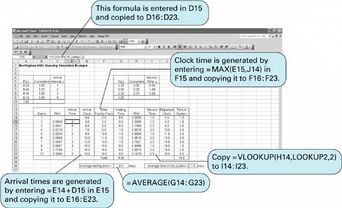
This process of selecting random numbers and generating arrival intervals and service times continues until 10 batch arrivals have been simulated, as shown in Table 14.7.

Once the simulation is complete, we can compute operating characteristics from the simulation results, as follows:

However, as in our previous example, these results must be viewed with skepticism. Ten trials of the system do not ensure steady-state results. In general, we can expect a considerable difference between the true average values and the values estimated from only 10 random draws. One reason is that we cannot be sure that the random numbers we selected in this example replicated the actual probability distributions because we used so few random numbers. The stream of random numbers that was used might have had a preponderance of high or low values, thus biasing the final model results. For example, of nine arrivals, five had interarrival times of 1 day. This corresponds to a probability of .55 (i.e., 5/9); however, the actual probability of an arrival interval of 1 day is .20 (from Table 14.5). This excessive number of short interarrival times (caused by the sequence of random numbers) has probably artificially inflated the operating statistics of the system.

[Page 625]

As the number of random trials is increased, the probabilities in the simulation will more closely conform to the actual probability distributions. That is, if we simulated the queuing system for 1,000 arrivals, we could more reasonably expect that 20% of the arrivals would have an interarrival time of 1 day.

An additional factor that can affect simulation results is the starting conditions. If we start our queuing system with no batches in the system, we must simulate a length of time before the system replicates normal operating conditions. In this example, it is logical to start simulating at the time the vat starts operating in the morning, especially if we simulate an entire working day. Some queuing systems, however, start with items already in the system. For example, the dyeing facility might logically start each day with partially completed batches from the previous day. In this case, it is necessary to begin the simulation with batches already in the system.

A factor that can affect simulation results is the starting conditions .

By adding a second random variable to a simulation model, such as the one just shown, we increase the complexity and therefore the manual operations. To simulate the example in Table 14.7 manually for 1,000 trials would require several hours. It would be far preferable to perform this type of simulation on a computer. A number of mathematical computations would be required to determine the various column values of Table 14.7, as we will demonstrate in the Excel spreadsheet simulation of this example in the next section.

Computer Simulation of the Queuing Example with Excel

The simulation of the dyeing process at Burlingham Mills shown in Table 14.7 can also be done in Excel. Exhibit 14.6 shows the spreadsheet simulation model for this example.

Exhibit 14.6.

[Page 626]

The stream of random numbers in column C is generated by the formula = RAND (), used in the ComputerWorld examples in Exhibits 14.2 through 14.5. (Notice that for this computer simulation, we have changed our random numbers from whole numbers to numbers between 0.0 and 1.0.) The arrival times are generated from the cumulative probability distribution of arrival intervals in cells B6:C9 . This array of cells is renamed "Lookup1" because there are two probability distributions in the model. The formula = VLOOKUP(C15, Lookup1,2 ) is entered in cell D15 and copied to cells D16:D23 to generate the arrival times in column D. The arrival clock times are computed by entering the formula = E14+D15 in cell E15 and copying it to cells E16:E23 .

Management Science Application: Simulating the Israeli Army Recruitment Process

Israel has compulsory army service starting at age 18. Candidates are examined while they are still in high school, a year before their recruitment. Prior to 1995 the examinations were conducted at six recruitment offices around the country. Each office included five major testing stations , where candidates were required to go through 2 days of examinations. The first day a candidate went through an admissions station, a premed station, and then a psychometric exam. Several weeks later the candidate would be scheduled for a second visit that included a personal interview and standard medical exam. More than 70% of the candidates did not finish the examination process during the 2 scheduled days and had to return for additional visits to finish all the tests. The recruitment offices were overcrowded, and staff worked at 100% capacity. Candidates spent over 40% of their time in the recruitment offices waiting in lines, and the average station waiting time was 30 minutes. This problem of overcrowding and delays was expected to get worse because of Israel's population growth from immigration (about 20%) during the 1990s. Possible solutions being considered included building an additional recruitment office and adding more personnel and staff.

A team was assigned to examine the recruitment process and overcrowding problem, with goals of finding a more cost-effective solution than building new facilities and adding personnel, and providing candidates with faster service, specifically reducing the number of extra visits. Preliminary analysis indicated that areas of improvement included the sequencing of the stations and the scheduling of the psychometric exam. The team created a simulation model to examine the various queuing situations that existed and the candidate flows through the system. The simulation model was used to analyze bottleneck situations and to evaluate possible alternatives, including changing the arrival patterns at stations, changing the way the psychometric test was administered, and looking at different possible routes through the process. After a year, a new recruiting configuration was developed, using the simulation model. A new computer system was installed that eliminated the use of personal files and thus saved wasted time for files to be physically transported between stations. A computerized routing system using bar codes assigned to candidates upon admission routed candidates to the stations with the shortest waiting times. The psychometric exam was computerized, thus eliminating the need to wait until examining rooms filled or emptied and to collect paper test results. Candidates' arrival times were evenly distributed during the morning.

The new system was implemented in 1995 in the Haifa office with successful results almost identical to those predicted by the simulation model. Ninety-nine percent of all candidates were able to complete all their tests in 1 day, in an average of 4 hours. Average station waiting time was reduced to 5 minutes. With the same workforce and facilities, throughput more than doubled . The new system was subsequently implemented in the five other recruiting offices with similar results. The two biggest offices in Tel Aviv were eventually merged, thus eliminating an office. This savings alone covered the cost of the entire project. Savings included $3.3 million for the closed offices plus $350,000 annually for reduced costs, including personnel and office expenses.

Source: O. Shtrichman, R. Ben-Haim, and M. Pollatschek, "Using Simulation to Increase Efficiency in an Army Recruitment Office," Interfaces 31, no. 4 (JulyAugust 2001): 6170.

[Page 627]

A batch of yarn can enter the dyeing facility as soon as it arrives (in column E) if there is not another batch being dyed or as soon as any batches being dyed or waiting to be dyed have departed the facility (column J). This clock time is computed by entering the formula = MAX(E15, J14 ) in cell F15 and copying it to cells F16:F23 . The waiting time is computed with the formula = F14-E14 , copied in cells G14:G23 .

A second set of random numbers is generated in column H by using the RAND () function. The service times are generated in column I from the cumulative probability distribution in cells H6:I8 , using the "Lookup" function again. In this case the array of cells in H6:I8 is named "Lookup2," and the service times in column I are generated by copying the formula = VLOOKUP(H14, Lookup2,2 ) in cells I14:I23 . The departure times in column J are determined by using the formula = F14+I14 copied in cells J14:J23 , and the "Time in System" values are computed by using the formula = J14-E14 , copied in cells K14:K23 .

The operating statistic, average waiting time, is computed by using the formula = AVERAGE(G14:G23 ) in cell G26, and the average time in the system is computed with a similar formula in cell L26. Notice that both the average waiting time of 0.4 days and the average time in the system of 1.9 days are significantly lower than the simulation conducted in Table 14.7, as we speculated they might be.