Appendix D: Markov Chains | Six Sigma and Beyond: Statistics and Probability, Volume III

In this appendix, we construct a probability model for a sequence of events that is a generalization of Bernoulli trials. Recall that Bernoulli trials are independent events and that the probability of success is constant from trial to trial. We generalize this model in two ways. First, we permit the number of possible outcomes to be some positive integer k where k 2. Thus we no longer can speak only of success or failure at a trial. Let A ₁ ,A ₂ ,...,A _k denote those possible outcomes. Second, we drop the assumption that the trials are independent events and introduce a certain amount of dependence. A large share of the interesting random variables in the social sciences as well as in the financial and engineering worlds are variables that are observed at regular time intervals over a given period of time. Very often those variables are not independent. For example, the price of a given individual stock may vary from week to week in a random manner, but its price during one week will usually depend rather heavily on what its price was during the preceding week. As another illustration, if a random variable represents the number of items, out of a set of n learned items, that will be recalled after, say, t time intervals have elapsed, then the value of that variable will certainly depend on how many items were recalled after t - 1 time intervals.

In some problems of the preceding type, the dependence is a local one in the sense that the value of the random variable at the end of t time intervals depends on its value at the end of t - 1 time intervals but not on any earlier time interval values. This would not usually be true, however, for the stock market because many buyers look at the past performance of a stock, and not merely at its price last week, in determining whether to buy it this week. In this section, we consider this special model in which the dependence of a random variable on earlier random variables extends only to the immediately preceding one. Thus we assume that the probability of outcome A _j occurring at a given trial depends on what outcome occurred at the immediately preceding trial but on no others.

Let P _ij denote the probability that outcome A _j will occur at a given trial if outcome A _i occurred at the immediately preceding trial. The possible outcomes A ₁ ,A ₂ ,...,A _k are called the states of the system. Thus P _ij is the probability of going from state A _i to state A _j at the next trial of the sequence. A sequence of experiments of the preceding type is called a Markov sequence or a Markov chain.

It should be noted that a Bernoulli sequence is a special case of a Markov sequence in which there are only two states A ₁ and A ₂ corresponding to success and failure and in which P ₁₁ = p, P ₁₂ = q, P ₂₁ = p, and P ₂₂ = q.

The probabilities P _ij , which are called transition probabilities, are usually displayed in matrix form as follows :

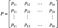
These probabilities apply to the system at any point in time. They express the probability relationship that exists at two neighboring time points, regardless of the chosen point in time.

The preceding probabilities are one-step transition probabilities. There are, however, also two-step and more generally n-step transition probabilities. A two-step transition probability, denoted by P _ij ⁽²⁾ , is the probability that the system will be in state A _j two time intervals later if it is now in state A _i . Formulas for expressing multiple-step transition probabilities in terms of one-step probabilities can be obtained by using matrix methods and the rules of probability. For example, to obtain a formula for P _ij ⁽²⁾ , we proceed as follows.

To arrive at A _j from A _i in exactly two steps, we must first go from A _j to A _r , where r is one of the integers 1,2,...,k and then go from A _r to A _j at the next step. The probability of doing this is P _ir P _rj . Since there are k mutually exclusive ways in which the desired event can occur corresponding to r = 1,2,...,k, the sum of those probabilities must be the value of P _ij ⁽²⁾ , Hence, we have the formula

(1)

Now consider the evaluation of P ² , that is, of the matrix product

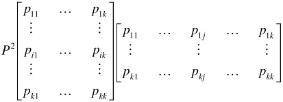
To obtain the element in the ith row and jth column of P ^2, it is necessary to multiply the ith row vector in the first matrix by the jth column vector in the second matrix. This gives the vector product

P _i1 P _1j + P _i2 P _2j +...+ P _ik P _kj

But this is the same as the expression defining P _ij ⁽²⁾ in (1); hence, it follows that P ² is the matrix whose typical element is P _ij ⁽²⁾ . We may express this relationship by writing

(2)

This shows that the two-step transition probabilities may be obtained by merely multiplying the one-step transition probability matrix by itself. In a similar manner, it follows that the n-step transition probabilities, p _ij ⁽ⁿ⁾ , are given by the relationship

p ⁿ = [p _ij ⁽ⁿ⁾ ]

As an illustration of a Markov chain, we consider a problem related to politics. Suppose that of the sons of Republican fathers, 60 percent vote Republican, 30 percent vote Democratic, and 10 percent vote Socialist; of the sons of Democratic fathers, 60 percent vote Democratic, 20 percent vote Republican, and 20 percent vote Socialist; of the sons of Socialist fathers, 50 percent vote Socialist, 40 percent vote Democratic, and 10 percent vote Republican. With this information, and assuming that the Markov chain properties hold true, we wish to perform the following:

Write down the transition matrix.
Calculate the two-step transition matrix.
Determine the probability that the grandson of a Republican man will vote Democratic.
Determine the same probability for a great-grandson.

Example:

Using the order Republican, Democrat, Socialist, the transition matrix is
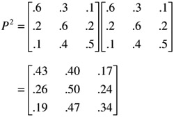
By using formula (2)
The answer here is given by P ₁₂ ⁽²⁾ ; hence, picking out the element in the first row and second column of P ² ,we obtain P ₁₂ ⁽²⁾ = .40.
Here we need the element P ₁₂ ⁽³⁾ , which can be obtained by multiplying the first row vector of P by the second column vector of P ² . This gives

(.6)(.40) + (.3)(.50) + (.1)(.47) = .437

In the preceding problem, suppose that the proportions of Republicans, Democrats, and Socialists in a community are given by the row vector A = [a ₁ a ₂ a ₃ ], where a ₁ + a ₂ + a ₃ = 1. Then the matrix product

is a row vector whose components give the proportions of Republicans, Democrats, and Socialists in the first generation of offspring (sons). For example, the first component in this product, namely

a ₁ P ₁₁ + a ₂ P ₂₁ + a ₃ P ₃₁

gives the probability that a first generation offspring will be a Republican, because it is the sum of the probabilities of the mutually exclusive ways in which a son will become a Republican. He may start with a Republican father and then become a Republican; or he may start with a Democratic father and then become Republican; or he may start with a Socialist father and then become a Republican. This works similarly for the other two components. In a similar manner, if we wish to calculate the proportions of male offspring who will be Republicans, Democrats, or Socialists at the nth generation, we merely need to calculate the matrix product AP ⁿ .

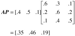
As an illustration, suppose that the preceding initial proportions are given by the row vector A = [.4 .5 .1]. Then after one generation the proportions become

After two generations, the proportions become

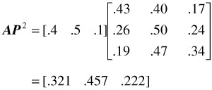
It would be interesting to carry these calculations further for succeeding generations to observe whether these proportions approach some fixed values. Calculating high powers of a matrix requires high-speed computing equipment and may be very expensive. Fortunately, however, there exists a mathematical theorem that tells us what happens to the transition probabilities in a Markov chain as n becomes increasingly large, without the necessity of extensive calculations. This theorem, which we do not prove , can be expressed as follows:

Theorem. As n ’ ˆ each row vector of P _n approaches the probability vector X that is a solution of the matrix equation XP = X.

It is easy to show that if P is a transition probability matrix, which implies that its elements are nonnegative and that the sum of the elements in any row is 1, then P ⁿ will also be a matrix of this type. Our theorem therefore states that the resulting transition probabilities are the same for all rows of the matrix.

As an illustration, we compute this transition matrix, which is often called the limiting transition matrix, for the preceding political problem. The equation that needs to be solved is the following one:

Multiplying the matrices on the left and equating components on both sides we obtain

.6x ₁ + .2x ₂ + .1x ₃ = x ₁

.3x ₁ + .6x ₂ + .4x ₃ = x ₂

.1x ₁ + .2x ₂ + .5x ₃ = x ₃

These equations are equivalent to the set

-.4x ₁ + .2x ₂ + .1x ₃ = 0

.3x ₁ - .4x ₂ + .4x ₃ = 0

.1xj + .2x ₂ - .5x ₃ = 0

They simplify to

-4x ₁ + 2x ₂ + x ₃ = 0

3x ₁ - 4x ₂ + 4x ₃ = 0

x ₁ + 2x ₂ - 5x ₃ = 0

Since the solution to our problem requires that X be a probability vector, we must have x ₁ + x ₂ + x ₃ = 1. The solution of the preceding equations that also satisfies this restriction is readily seen to be given by

Our theorem then states that as n ’ ˆ , the elements of P ⁿ approach the elements of the matrix

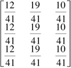
Now let us calculate the long-run proportions of Republicans, Democrats, and Socialists. Just as was done earlier to obtain the first- and second-generation proportions, this can be accomplished by calculating the product of the row vector [.4 .5 .1] and the matrix just obtained. This gives

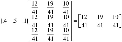
It should be observed that since the rows of the limiting transition matrix are all equal and the elements of the row vector A sum to 1, it follows that the result of this type of matrix product must be a row of the limiting transition matrix. Hence, the preceding solution

gives the proportions of Republicans, Democrats, and Socialists that will be realized in the long run if the transition probabilities do not change over time. Incidentally, this also shows that the initial set of proportions, .4, .5, and .1, has no effect on the long-run set of proportions.

The preceding result, showing that the limiting proportions are the same as the limiting values of the transition probabilities, is quite general. It did not depend on the particular numbers used in the illustration. Thus it is true in general that the initial proportions in any problem have no effect on the long-run proportions. Those proportions depend only on the nature of the transition probabilities.