Chapter 48: Incorporating Qualitative Factors into Multiple Regression

• How can I predict quarterly U.S. auto sales?

• How can I predict U.S. presidential elections?

• Is there an Excel function I can use to easily make forecasts from a multiple regression equation?

In our first example of multiple regression in Chapter 47, “Incorporating Qualitative Factors into Multiple Regression,” we forecasted the monthly cost of plant operations by using the number of units of each product manufactured at the plant. Because we can quantify exactly the amount of a product produced at the plant, we can refer to the units produced of Product A, Product B, and Product C as quantitative independent variables. In many situations, however, independent variables can’t be easily quantified. In this chapter, we’ll look at ways to incorporate qualitative factors such as seasonality, gender, or the party of a presidential candidate into a multiple regression analysis.

• How can I predict quarterly U.S. auto sales?

• Suppose we want to predict quarterly U.S. auto sales to determine whether the quarter of the year impacts auto sales. We’ll use the data in the file Auto.xlsx, shown in Figure 48-1 on the next page. Sales are listed in thousands of cars, and GNP is in billions of dollars.)

  
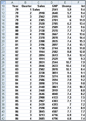
  Figure 48-1: Auto sales data

• You might be tempted to define an independent variable that equals 1 during the first quarter, 2 during the second quarter, and so on. Unfortunately, this approach would force the fourth quarter to have four times the effect of the first quarter, which might not be true. The quarter of the year is a qualitative independent variable. To model a qualitative independent variable, we create an independent variable (called a dummy variable) for all but one of the qualitative variable’s possible values. (It is arbitrary which value you leave out. In this example, I chose to omit Quarter 4.) The dummy variables tell you which value of the qualitative variable occurs. Thus, we’ll have a dummy variable for Quarter 1, Quarter 2, and Quarter 3 with the following properties:

  • Quarter 1 dummy variable equals 1 if the quarter is Quarter 1, and 0 if otherwise.

  • Quarter 2 dummy variable equals 1 if the quarter is Quarter 2, and 0 if otherwise.

  • Quarter 3 dummy variable equals 1 if the quarter is Quarter 3, and 0 if otherwise.

• A Quarter 4 observation will be identified by the fact that the dummy variables for Quarter 1 through Quarter 3 equal 0. You can see why we don’t need a dummy variable for Quarter 4. In fact, if we include a dummy variable for Quarter 4 as an independent variable in our regression, Microsoft Office Excel 2007 returns an error message. The reason we get an error is that if an exact linear relationship exists between any set of independent variables, Excel must perform the mathematical equivalent of dividing by 0 (an impossibility) when running a multiple regression. In our situation, if we include a Quarter 4 dummy variable, every data point satisfies the following exact linear relationship:

   (Quarter 1 Dummy)+(Quarter 2 Dummy)+(Quarter 3 Dummy)+(Quarter 4 Dummy)=1

  Note 

  An exact linear relationship occurs if there exists constants c0, c1, … cN, such that for each data point c0 + c1x1 + c2x2 + … cNxN = 0. Here x1, … xN are the values of the independent variables.

• To create our dummy variable for Quarter 1, I copied from G12 to G13:G42 the formula IF(B12=1,1,0). This formula places a 1 in column G whenever a quarter is the first quarter, and places a 0 in column G whenever the quarter is not the first quarter. In a similar fashion, I created dummy variables for Quarter 2 (in H12:H42) and Quarter 3 (in I12:I42). You can see the results of the formulas in Figure 48-2.

  
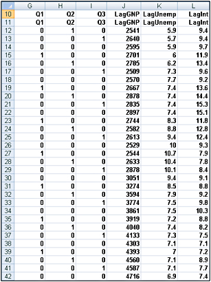
  Figure 48-2: Using dummy variables to track the quarter in which a sale occurs

• In addition to seasonality, we’d like to use macroeconomic variables such as gross national product (GNP, in billions of 1986 dollars), interest rates, and unemployment rates to predict car sales. Suppose, for example, that we are trying to estimate sales for the second quarter of 1979. Because values for GNP, interest rate, and unemployment rate aren’t known at the beginning of the second quarter 1979, we can’t use second quarter 1979 GNP, interest rate, and unemployment rate to predict Quarter 2 1979 auto sales. Instead, we’ll use the values for GNP, interest rate, and unemployment rate lagged one quarter to forecast auto sales. By copying from J12 to J12:L42 the formula =D11, we create the lagged value for GNP, the first of our macroeconomic independent variables. For example, the range J12:L12 contains GNP, unemployment rate, and interest rate for the first quarter of 1979.

• We can now run our multiple regression by clicking Data Analysis on the Data tab, and then selecting Regression in the Data Analysis dialog box. We use C11:C42 as the Input Y Range, G11:L42 as the Input X Range, check the Labels box (row 11 contains labels), and also check the Residuals box. After clicking OK, we obtain the output, which you can see in the Regression worksheet and in Figures 48-3 through 48-5.

  
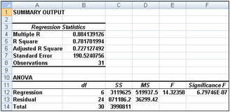
  Figure 48-3: Summary output and ANOVA table for auto sales data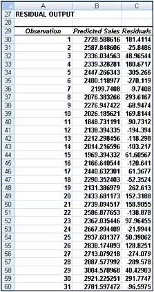

  
  Figure 48-5: Residuals for the auto sales data

• In Figure 48-4, we can see that the equation (equation 1) used to predict quarterly auto sales is as follows:

   Predicted quarterly sales=3154.7+156.833Q1+379.784Q2+203.03 6Q3+.174(LAGGNP in billions)−93.83(LAGUNEMP)−73.91(LAGINT)

• Also in Figure 48-4, we see that each independent variable has a p-value less than or equal to 0.15. We can conclude that all independent variables have a significant effect on quarterly auto sales. We interpret all coefficients in our regression equation ceteris paribus (which means that each coefficient gives the effect of the independent variable after adjusting for the effects of all other variables in the regression).

  
  Figure 48-4: Coefficient information for auto sales regression

• Here’s an interpretation of each coefficient:

  • A $1 billion increase in last quarter’s GNP increases quarterly car sales by 174.

  • An increase of 1 percent in last quarter’s unemployment rate decreases quarterly car sales by 93,832.

  • An increase of 1 percent in last quarter’s interest rate decreases quarterly car sales by 73,917.

• To interpret the coefficients of the dummy variables, we must realize that they tell us the effect of seasonality relative to the value left out of the qualitative variables. Therefore:

  • In Quarter 1, car sales exceed Quarter 4 car sales by 156,833.

  • In Quarter 2, car sales exceed Quarter 4 car sales by 379,784.

  • In Quarter 3, car sales exceed Quarter 4 car sales by 203,036.

• We find that car sales are highest during the second quarter (April through June; tax refunds and summer are coming) and lowest during the third quarter (October through December; why buy a new car when winter salting will ruin it?).

• From the Summary output shown in Figure 48-3, we can learn the following:

  • The variation in our independent variables (macroeconomic factors and seasonality) explains 78 percent of the variation in our dependent variable (quarterly car sales).

  • The standard error of our regression is 190,524 cars. We can expect around 68 percent of our forecasts to be accurate within 190,524 cars and about 95 percent of our forecasts to be accurate within 381,048 cars (2*190,524).

  • There are 31 observations used to fit the regression.

• The only quantity of interest to us in the ANOVA table in Figure 48-3 is the significance (0.00000068). This measure implies that there are only 6.8 chances in 10,000,000 that, taken together, all of our independent variables are useless in forecasting car sales. Thus, we can be quite sure that our independent variables are useful in predicting quarterly auto sales.

• Figure 48-5, on the next page, shows, for each observation, the predicted sales and residual. For example, for the second quarter of 1979 (observation 1), predicted sales from equation 1 are 2728.6 thousand and our residual is 181,400 cars (2910–2728.6). Note that no residual exceeds 381,000 in absolute value, so we have no outliers.

• How can I predict U.S. presidential elections?

• When asked which factors drive presidential elections, presidential advisor James Carville said, “It’s the economy, stupid.” Yale economist Roy Fair showed that Carville was correct in thinking that the state of the economy has a large influence on the results of presidential elections. Fair’s dependent variable (see the file President.xlsx, shown in Figure 48-6) for each election (1916 through 2004) was the percentage of the two party vote (ignoring votes received by third party candidates) that went to the incumbent party. He tried to predict the incumbent party’s percentage of the two-party vote by using independent variables such as:

  • Party in power. In our data, we use 1 to denote when the Republican party was in power and 0 to denote when the Democratic party was in power.

  • Percentage growth in GNP during the first nine months of the election year.

  • Absolute value of the inflation rate during the first nine months of the election year. We use the absolute value because either a positive or a negative inflation rate is bad.

  • Number of quarters during the last four years in which economic growth was strong. Strong economic growth is defined as growth at an annual level of 3.2 percent or more.

  • Length of time an incumbent party had been in office. Fair used 0 to denote one term in office, 1 for two terms, 1.25 for three terms, 1.5 for four terms, and 1.75 for five terms or more. This definition implies that each term after the first term in office has less influence on the election results than the first term in office.

  • Elections during wartime. The elections in 1920 (World War I), 1944 (World War II), and 1948 (World War II was still underway in 1945) were defined as wartime elections. (Elections held during the Vietnam war were not considered to be wartime elections.) During wartime years, the variables related to quarters of good growth and inflation were deemed irrelevant and were set to 0.

  • The current president running for re-election. If this is the case, this variable is set to 1; otherwise, this variable is set to 0. In 1976, Gerald Ford was not considered a president running for re-election because he was not elected either as president or as vice-president.

  
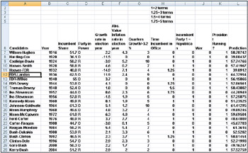
  Figure 48-6: Presidential election data

  Note 

  Our data comes from Roy Fair’s excellent book Predicting Presidential Elections and Other Things (Stanford University Press, 2002).

• I’ve attempted to use the data from the elections from 1916 through 2000 to develop a multiple regression equation that can be used to forecast future presidential elections. I saved the 2004 election as a “validation point.” When fitting a regression to data, it’s always a good idea to hold back some of your data for use in validating your regression equation. Holding back data allows you to determine whether your regression equation can do a good job of forecasting data it hasn’t seen. Any forecasting tool that poorly forecasts data it hasn’t seen should not be used to predict the future.

• To run the regression, click Data Analysis in the Analysis group on the Data tab, and then select the Regression tool in the Data Analysis dialog box. I used C6:C28 as the Input Y Range and E6:K28 as the Input X Range. I also checked the Labels box (row 6 contains labels) and the Residuals box. I’ve placed the output in the Results worksheet, which you can see in Figures 48-7 and 48-8 on the next page.

  
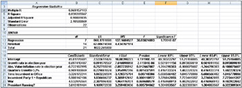
  Figure 48-7: Regression output for predicting presidential elections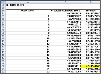

  
  Figure 48-8: Presidential election residuals

• In Figure 48-7, you can see that the p-value for each independent variable is much less than 0.15, which indicates that each of our independent variables is helpful in predicting presidential elections. We can predict elections using an equation such as the following (equation 2):

   Predicted presidential election percentage=45.813+.70GROWTH-.72ABSINF+.91GOODQUARTERS- 3.33TIMEINCUMB+5.5REP+4.53WAR+3.81PRESRUNNING

• The coefficients of the independent variables can be interpreted as follows (after adjusting for all other independent variables used in equation 2):

  • A 1 percent increase in the annual GNP growth rate during an election year is worth 0.7 percent to the incumbent party.

  • A 1 percent deviation from the ideal (0 percent inflation) costs the incumbent party 0.72 percent of the vote.

  • Every good quarter of growth during an incumbent’s term increases his (maybe her someday soon!) vote by 0.91 percent.

  • Relative to having one term in office, the second term in office decreases the incumbent’s vote by 3.33 percent, and each later term decreases the incumbent’s vote by 0.25*(3.33 percent)=0.83 percent.

  • A Republican has a 5.5 percent edge over a Democrat.

  • A wartime incumbent president has a 4.53 percent edge over his opponent.

  • A sitting president running for re-election has a 3.81 percent edge over his opponent.

• We find that 94 percent of the variation in the percentage received by an incumbent in a presidential election is explained by our independent variables. This is amazing! We have not mentioned whether the candidates are “good” or “bad” candidates. Our standard error of 2.10 percent indicates that about 95 percent of our forecasts will be accurate within 4.2 percent. From our residuals, shown in Figure 48-8, we find the only election outlier to be the 1992 Clinton-Bush election. George Bush Sr. received 4.31 percent less than our model predicted, which probably indicates that Bill Clinton was a great campaigner!

• Is there an Excel function I can use to easily make forecasts from a multiple regression equation?

• It’s tedious to make forecasts using an equation such as equation 2, but the Excel TREND function makes it easy to generate forecasts from a multiple regression. You don’t even have to run a regression with the Data Analysis command.

• To illustrate the use of the TREND function, I’ll describe how to generate forecasts for the 1916 through 2004 elections using data from only the 1916 through 2000 elections. Begin by selecting the cell range (in our example, L7:L29 in the Data worksheet) where you want your forecasts to go. With the pointer in the first cell of this range (cell L7 in our example), enter the formula TREND(C7:C28,E7:K28,E7:K29). Next, press Ctrl+Shift+Enter. You’ll now see the forecast for each election, generated in cells L7:L29. Note that the forecast for the 2004 election (using data only through 2000) was that Bush would receive 57.5 percent of the vote. Thus, Bush’s share of the popular vote was an outlier on the low side. Maybe this was due to the unpopularity of the Iraq War.

• The TREND function is an example of an array function. I’ll provide a more complete discussion of array functions in Chapter 74, “Array Functions and Formulas.” For now, here is some background about array functions:

  • Before entering an array function, you must always select the cell range in which you want the results of the array function to be located.

  • Instead of pressing Enter to perform the calculation, you must press Ctrl+Shift+Enter to complete the entry of an array function.

  • After entering an array function, you’ll see a curly bracket in the formula bar when you select a cell in which the array function’s results are located. This bracket indicates that the results in the cell were computed with an array function.

  • You can’t modify data in any part of a range created by an array function.

Note 

Problems that you can work with to learn more about multiple regression are available at the end of Chapter 49.