Section 4.1. Formatting Cell Values | Excel 2007 for Starters: The Missing Manual

4.1. Formatting Cell Values

Cell value formatting is one aspect of worksheet design you don't want to ignore, because the values Excel stores can differ wildly from the numbers that it displays in the worksheet, as shown in Figure 4-1. In many cases, it makes sense to have the numbers that appear in your worksheet differ from Excel's underlying values, since a worksheet that's displaying numbers to, say, 13 decimal places, can look pretty cluttered.

Figure 4-1. Each of the cells B2, B3, and B4 contains the same number: 5.18518518518519. In the Formula bar, Excel will always display the exact number it's storing, as you see here with cell B2. However, in the worksheet itself, each cell's appearance differs depending on how you've formatted it.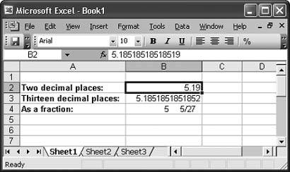

To format a cell's value, follow these steps:

Select the cells you want to format.
You can apply formatting to individual cells or to a collection of cells. Usually, you'll want to format an entire column at once, because all the values in a column typically contain the same type of data. Remember, to select a column, you simply need to click the column header (the gray box at the top with the column letter).
Note: Technically, your average numeric column contains two types of data: the values you're storing within the actual cells and the column title in the topmost cell (where the title text is). However, you don't need to worry about unintentionally formatting the column title because number formats are applied only to numeric cells (cells that contain dates, times, or numbers). Excel doesn't use the number format for the column title cell because the column title cell contains text.
Select Format Cells, or just right-click the selection and choose Format Cells.
Set the format options you want, and then click OK to apply them.
The options in the Number tab let you choose how Excel translates the cell value into a display value. (Number formatting choices are covered in the next section on Section 4.1.1.) The Alignment, Font, Border, and Patterns tabs are for cell appearance formatting, which is covered later in this chapter. (The Protection tab lets you hide formulas and lock your worksheet to prevent changes.)

Note: Once you apply formatting to a cell, it retains that formatting even if you clear the cell's contents (by selecting it and pressing Delete). In addition, formatting is part of a cell copy, so if you copy cell A1 to cell A2, Excel copies the formatting right along with the content. Formatting includes both cell value formatting and cell appearance.The only way to remove the formatting is to highlight the cell and select Edit

Clear

Formats. This command removes the formatting, restoring the cell to its original, General number format (which youll learn more about next), but doesn't remove any of the cell's content.

Figure 4-2. The Format Cells dialog box provides one-stop shopping for cell value and cell appearance formatting.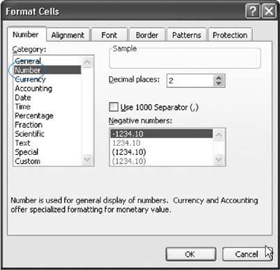

4.1.1. Formatting Numbers

The Number tab in the Format Cells dialog box lets you control how Excel displays numeric data in a cell. Excel gives you a lengthy list of predefined formats (shown in Figure 4-3), and it also lets you design your own formats. Remember, Excel uses number formats when the cell contains numeric information only. Otherwise, Excel simply ignores the number format (although the format is still there; Excel will use it if you change the cell content to a number, date, or time).

A good way to learn about the different number formats is to choose a new number format (such as Currency) from the Format Cells dialog box's Category list, as shown in Figure 4-3. When you do so, the Sample area of the dialog box shows how the number will be displayed if you apply that format. Excel also offers additional options you can use to customize the format. For example, if you choose the Currency format, Excel offers a list of currency symbols you can pick fromeverything from dollars to kroner. To apply a format, just select the format and then click OK.

Figure 4-3. Here, the formatting category is Currency. The Sample area shows how the cell value333will appear in the worksheet: as $333.00, with two decimal places and a dollar sign. Clicking the Symbol list lets you choose another currency symbolfor example, English pounds or Jamaican dollars. To apply the format, click OK.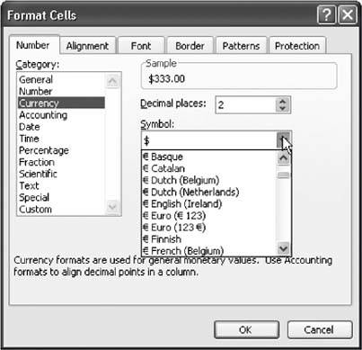

When you create a new spreadsheet, every cell starts out with the same number format: General. This format comes with a couple of basic rules:

If a number has any decimal places, Excel displays them, provided they fit in the column. If there are more decimal places than Excel can display, it leaves out the ones that don't fit. (It rounds up the last displayed digit, when appropriate). If you change a column width, Excel automatically adjusts the number of digits it displays.
Excel removes leading and trailing zeros. Thus, 004.00 becomes 4. The only exception to this rule occurs with numbers between -1 and 1, which retain the 0 before the decimal point. For example, Excel displays the number .42 as 0.42.

As you saw in Chapter 2, the way you type in a number can change a cell's formatting. For example, if you type in a number with a currency symbol, the number format of the cell changes automatically to Currency. Similarly, if you type in three numbers separated by dashes (-) or backward slashes (/), Excel assumes you're typing in a date and adjusts the number format to Date.

It's nice that Excel tries to be so helpfulbut some things are best left up to people, not software. Rather than rely on this automatic process (especially when currency is involved), it's far better just to type in ordinary numbers and set the formatting explicitly for the whole column. This approach prevents you from having different formatting in different cells (which can confuse even the sharpest spreadsheet reader), and it makes sure you get exactly the formatting and precision you want. You can apply formatting to the column before or after you type in the numbers. And it doesn't matter if a cell is currently empty; Excel still keeps track of the number format you've applied.

Most of the spreadsheets you'll create will probably contain numbers in some form or fashion. So the following sections give a quick tour of the predefined number formats available on the Number tab in the Format Cells dialog box. Figure 4-4 gives you an overview of how different number formats affect similar numbers.

4.1.1.1. General

The General format is Excel's standard number format; it applies no special formatting other than the basic rules described at the beginning of this chapter. General is the only number format (other than Text) that doesn't limit your data to a fixed number of decimal places. That means if you want to display numbers that differ wildly in precision (like 0.5, 12.334, and 0.120986398), you can do so using the General format. On the other hand, if your numbers have a similar degree of precision (for example, if you're logging the number of hours of TV you watch each day), Number format makes more sense.

Figure 4-4. Each column contains the same list of numbers. Although this worksheet shows an example for each number format (except the less-frequently-used scientific and time categories), it doesn't show all your options. Each number format has its own settingslike the number of decimal placesthat affect how Excel displays data.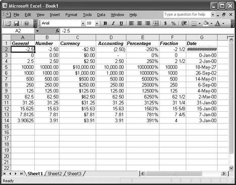

4.1.1.2. Number

The Number format is like the General format, but with three refinements. First, the Number format uses a fixed number of decimal places (which you set). That means that the decimal point always lines up (assuming you've formatted an entire column). The Number format also lets you use commas as a separator between groups of three digits, which is handy if you're working with really long numbers. Finally, you can choose to have negative numbers displayed with the negative sign, in parentheses, or in red lettering.

4.1.1.3. Currency

The Currency format closely matches the Number format, with two differences. First, you can choose a currency symbol (like the dollar sign, pound symbol, Euro symbol, and so on) from an extensive list; when you do, Excel automatically displays the currency symbol before the number. Second, the Currency format always includes commas. The Currency format also supports a fixed number of decimal places (chosen by you), and it lets you customize how negative numbers are displayed.

4.1.1.4. Accounting

The Accounting format is modeled on the Currency format. It also lets you choose a currency symbol, uses commas, and has a fixed number of decimal places. The difference is that the Accounting format uses a slightly different alignment. The currency symbol always appears at the far left of the cell (away from the number), and Excel always adds an extra space to pad the right side of the cell. Also, the Accounting format always shows negative numbers in parentheses, which is an accounting standard. Finally, Excel never shows the number 0 when using the Accounting format; instead of a zero, it displays a dash (-).

4.1.1.5. Percentage

The Percentage format displays fractional numbers as percentages. For example, if you type in 0.5, that translates to 50%. You can choose the number of decimal places to display.

There's one trick to watch out for with the Percentage format. If you forget to start your number with a decimal, Excel quietly "corrects" your numbers. For example, if you type 4 into a cell that uses the Percentage format, Excel interprets the 4 as 4%. As a result, it actually stores the value 0.04. A side effect of this quirkiness is that if you want to store percentages larger than 100%, you can't type them in as decimals. For example, to store 200%, you need to type in 200 (not 2.00).

4.1.1.6. Fraction

The Fraction format displays your number as a fraction instead of a number with decimal places. The Fraction format doesn't mean you have to type in the number as a fraction (although you can if you want by using the forward slash, like 3/4). Instead it means that Excel automatically converts any number you type in and displays it as a fraction. So, for example, to have 1/4 appear, you can either type in .25 or 1/4.

Lots of folks use the Fraction format for stock market quotes, but it's also handy for certain types of measurements (like weights, temperatures, and recipes). When using the Fraction format, Excel does its best to calculate the closest fraction, which depends on a few factors, including whether an exact match exists (typing in .5 will always get you 1/2, for example) and what type of precision level you've picked when selecting the Fraction formatting.

You can choose to have fractions with three digits (for example, 100/200), two digits (10/20), or just one digit (1/2), using the top three choices in the Type list. For example, if you type in the number 0.51, Excel shows it as 1/2 in one-digit mode, and the more precise 51/100 in three-digit mode. In some cases, you may want all numbers to use the same denominator (the bottom number in the fraction) so that it's easy to compare different numbers. In this case, you can choose to show all fractions as halves (with a denominator of 2), quarters (a denominator of 4), eighths (8), sixteenths (16), tenths (10), and hundredths (100). For example, the number 0.51 would be shown as 2/4 if you chose quarters.

Tip: You might feel like pulling your hair out in tufts when you're trying to type a fraction into Excel, and Excel keeps converting your fraction to a date (both use slashes). To prevent this confusion, always start by typing 0 and then a space. For example, instead of typing 2/3, type in 0 2/3 (which means zero and two-thirds). If you have a whole number and a fraction, like 1 2/3, you'll also be able to duck the date confusion.

UP TO SPEED
The Relationship Between Formatting and Values

The format you choose for a number doesn't affect Excel's internal storage of that number. For example, if a cell contains the fraction 1/3, Excel stores this value as 0.333333333333333. (The exact number of decimal places varies, depending on the number you type in, due to the slight approximations computers need to make when converting fractional numbers into 0's and 1's.) When deciding how to format a cell, you can choose to show only two decimal places, in which case the number appears in your worksheet as 0.33. Or maybe you choose just one decimal place, in which case the number will simply be 0.3. In both cases, Excel still keeps the full fifteen or so decimal places on hand. To tell the difference between the displayed number and the real number that Excel stores behind the scenes, just move to the cell. Then look at the Formula bar, which always shows you the real deal.

Because there's a difference between the stored value and the displayed number, there may be some situations in which it looks like Excel is making a mistake. For example, imagine you have three cells, and each stores 0.333333333333333 but displays only 0.3. When you add these three cell values together, you won't end up with 0.3 + 0.3 + 0.3 = 0.9. Instead, you'll add the more precise stored values and end up with a number that's infinitesimally close to, but not quite, 1. Excel rounds this number up to 1.

Storing and displaying slightly different values is almost always the way you want Excel to work, because you know full well that if you add up 1/3 three times you end up with 1. But if you need to, you can change this behavior.

If you select Tools Options and then select the Calculate tab (or the Calculation tab, if youre using Excel 2002), you'll see a "Precision as displayed" checkbox. When you turn on this checkbox, Excel adjusts all the values in your current spreadsheet so that the (accurate) stored value matches the (loosey-goosey) displayed value. Because you can't reverse this change, Excel warns you and asks for a final confirmation when you try to apply the "Precision as displayed" setting.

4.1.1.7. Scientific

The Scientific format displays numbers using scientific notation, which is ideal if you ever find yourself needing to handle numbers that range widely in size (like 0.0003 and 300) in the same column. Scientific notation displays the first non-zero digit of a number, followed by a fixed number of digits, and then indicates what power of 10 that number needs to be multiplied by to generate the original number. For example, 0.0003 becomes 3.00 10^-4 (displayed in Excel as 3.00E-04). The number 300, on the other hand, becomes 3.00 10² (displayed in Excel as 3.00E02). Scientistssurprise, surpriselike the Scientific format for doing things like recording experimental data or creating mathematical models to predict when an incoming meteor will graze Earth. Most of the rest of us can safely skip the Scientific format.

4.1.1.8. Text

Few people use the Text format for numbers, but it's certainly possible to do so. The Text format simply displays a number as though it were text, although you can still perform calculations with it. Excel shows the number exactly as it's stored internally, positioning it against the left edge of the column. You can get the same effect by placing an apostrophe before the number (although that approach won't let you use the number in calculations).

4.1.2. Formatting Dates and Times

To format dates and times, in the Format Cells dialog box (Format Cells), shown in Figure 4-5, choose Date or Time from the column on the left and then choose the format from the list on the right. Date and Time both provide a slew of options. You can use everything from compact styles like Sunday, March 13, 2005. You can choose a format that modifies the date's appearance depending on the regional settings of the computer viewing the Excel file (handy if you live in Baton Rouge and want your boss in Bangkok and your employees in Glasgow to view your worksheet), or you can choose a fixed date format. When using a fixed date format, you don't have to stick to the U.S. standard. Instead, choose the locale (geographic location) you want from the Locale listbox. Each localefrom Albanian to Vietnameseprovides its own set of customized date formats.

Figure 4-5. In a world of clock-watchers, it's no surprise that Excel offers dozens of different ways to format dates and times. You can choose between formats that modify the date's appearance depending on the regional settings of the computer viewing the Excel file, or you can choose a fixed date format from the Locale listbox.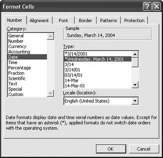

Time formats give you a similar range of options, including the ability to use a 12-hour or 24-hour clock, show seconds, show fractional seconds, and include the date information.

Excel offers two types of date and time formats:

Formats that take the regional settings of the computer you're using into account. With these formats, dates display differently depending on the computer that's running Excel. This choice is a good one because it lets everyone see dates just the way they want to, no matter where in the world they are. No more time-consuming Brits-vs.-Yanks arguments about whether the "real" way to order a date is month-day-year or day-month-year.
Formats that ignore the regional settings of individual computers. These formats define a fixed pattern for month, day, year, and time components, and display date-related information in exactly the same way on all computers. If you need to make sure a date is in a certain format, no ifs, ands, or buts, you should use this choice.

The first type (date and time formats that rely on a computer's regional settings) is the quickest to set. It includes just two date formats (a compact number-only format and a long, more descriptive format) and a single time format. You find these formats at the top of the Type list with an asterisk next to them.

Setting the second type (date and time formats that are independent of a computer's regional settings) takes a bit more doing. To choose one of these formats, you first select a geographical region from the Locale list, and then you select the appropriate date or time format. Some examples of locales include "English (United States)," "English (United Kingdom)," and "Arabic(Iraq)."

If you type in a date without specifically formatting the cell, Excel usually uses the short, region-specific date format. That means that the order of the month and year vary depending on the regional settings of your computer (or, if it's your bookie who's looking at your worksheet, your bookie's computer). But if you incorporate the month name (for example, January 1, 2005), instead of the month number (for example, 1/1/2005), Excel uses a compromise date format that includes a month abbreviation, like 1-Jan-2005.

Tip: You may remember from Chapter 2 that Excel stores a date internally as the cumulative number of days that have elapsed since a certain long-ago date that varies by operating system. If you're curious, you can take a peek at this internal number using the Format Cells dialog box. First, type in your date. Then, format the cell using one of the number formats (like General or Number). The underlying date number appears in your worksheet where the date used to be.

FREQUENTLY ASKED QUESTION
Just How Precise Are Excel Numbers, Anyway?

Can I type in a number with 10 decimal places? How about 20?

Here's a handy way to find out: type the fraction 0 2/3 into a cell, and then check the Formula bar, which shows you the number Excel has stored. Turns out Excel thinks of 2/3 as 0.666666666666667.

This test demonstrates that Excel limits you to about 14 significant digits, and that it rounds up the last digit. You may be slightly unnerved by the word "about," but in the binary world of computers, fractional numbers don't have a fixed number of digits and may just be approximations with very slight rounding errors. If you're interested, you can find one good (but technical) explanation of this phenomenon on Wikipedia (an online encyclopedia) at http://en.wikipedia.org/wiki/Floating_point.

Because Excel doesn't store fractions precisely as they exist in the world of real math, you may occasionally experience minor rounding errors in calculations with more than 14 significant digits. (Recall from high school math that the number of significant digits is the number of digits starting with the first non-zero digit (and ending with the last non-zero digit if there is no decimal point). Essentially, the significant digits hold all the information in your number.) This behavior shouldn't cause you to panicit's a limitation of nearly all computer software, based on the way that computers manipulate numbers. And seriously, how often are mere mortals concerned with that kind of precision, anyway?

4.1.3. Special Formats for Special Numbers

There are some types of numeric information that you wouldn't ever want to perform mathematical operations with. For example, it's hard to image a situation where you'd want to add or multiply phone numbers or Social Security numbers.

So when you're typing in these kinds of numbers, you can format them as plain old text. For example, you could type in the text (555) 123-4567 to represent a phone number. Because there are parentheses and a dash (-), Excel won't interpret this information as a number. Or, you could just precede your value with an apostrophe (') to explicitly tell Excel that it should be treated as text.

But whichever solution you choose, you're potentially creating more work for yourself. Why? Because you have to type in the parentheses and the dash (or the apostrophe) for each phone number you type in. You also increase the likelihood of creating inconsistently formatted numbers, especially if you're typing in a long list of them. For example, careful as you are, some phone numbers may end up in slightly similar but somewhat different formats, like 555-123-4567 and (555)1234567.

To avoid these problems, apply Excel's Special number format, as shown in Figure 4-6, which converts numbers into common patterns. And lucky you: one of the Type options in the Special number format is Phone Number (other formats are for Zip codes and Social Security numbers).

After you apply the special Phone Number format to a cell, all you do is type in a series of digits, such as 5551234567; Excel automatically converts the digits to the proper phone number style(555) 123-4567without your having to type in all those pesky parentheses and dashes.

The Special format is a good idea, but it's limited because Excel only provides a small set of special types that you can use. However, there's no reason you can't handle similar problems by creating your own custom formats, covered extensively in Excel: The Missing Manual.