Characteristics of Methods for Clustering Observations

Many simulation studies comparing various methods of cluster analysis have been performed. In these studies, artificial data sets containing known clusters are produced using pseudo-random-number generators. The data sets are analyzed by a variety of clustering methods, and the degree to which each clustering method recovers the known cluster structure is evaluated. Refer to Milligan (1981) for a review of such studies. In most of these studies, the clustering method with the best overall performance has been either average linkage or Ward's minimum variance method. The method with the poorest overall performance has almost invariably been single linkage. However, in many respects, the results of simulation studies are inconsistent and confusing.

When you attempt to evaluate clustering methods, it is essential to realize that most methods are biased toward finding clusters possessing certain characteristics related to size (number of members ), shape, or dispersion. Methods based on the least-squares criterion (Sarle 1982), such as k -means and Ward's minimum variance method, tend to find clusters with roughly the same number of observations in each cluster. Average linkage is somewhat biased toward finding clusters of equal variance. Many clustering methods tend to produce compact, roughly hyperspherical clusters and are incapable of detecting clusters with highly elongated or irregular shapes . The methods with the least bias are those based on nonparametric density estimation such as single linkage and density linkage.

Most simulation studies have generated compact (often multivariate normal) clusters of roughly equal size or dispersion. Such studies naturally favor average linkage and Ward's method over most other hierarchical methods, especially single linkage. It would be easy, however, to design a study using elongated or irregular clusters in which single linkage would perform much better than average linkage or Ward's method (see some of the following examples). Even studies that compare clustering methods using 'realistic' data may unfairly favor particular methods. For example, in all the data sets used by Mezzich and Solomon (1980), the clusters established by field experts are of equal size. When interpreting simulation or other comparative studies, you must, therefore, decide whether the artificially generated clusters in the study resemble the clusters you suspect may exist in your data in terms of size, shape, and dispersion. If, like many people doing exploratory cluster analysis, you have no idea what kinds of clusters to expect, you should include at least one of the relatively unbiased methods, such as density linkage, in your analysis.

The rest of this section consists of a series of examples that illustrate the performance of various clustering methods under various conditions. The first, and simplest example, shows a case of well-separated clusters. The other examples show cases of poorly separated clusters, clusters of unequal size, parallel elongated clusters, and nonconvex clusters.

Well-Separated Clusters

If the population clusters are sufficiently well separated, almost any clustering method performs well, as demonstrated in the following example using single linkage. In this and subsequent examples, the output from the clustering procedures is not shown, but cluster membership is displayed in scatter plots. The following SAS statements produce Figure 7.1:

  data compact;   keep x y;   n=50; scale=1;   mx=0; my=0; link generate;   mx=8; my=0; link generate;   mx=4; my=8; link generate;   stop;   generate:   do i=1 to n;   x=rannor(1)*scale+mx;   y=rannor(1)*scale+my;   output;   end;   return;   run;   proc cluster data=compact outtree=tree   method=single noprint;   run;   proc tree noprint out=out n=3;   copy x y;   run;   legend1 frame cframe=ligr cborder=black   position=center value=(justify=center);   axis1 minor=none label=(angle=90 rotate=0);   axis2 minor=none;   proc gplot;   plot y*x=cluster/frame cframe=ligr   vaxis=axis1 haxis=axis2 legend=legend1;   title 'Single Linkage Cluster Analysis';   title2 'of Data Containing Well-Separated,   Compact Clusters';   run;

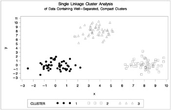
Figure 7.1: Data Containing Well-Separated, Compact Clusters: PROC CLUSTER with METHOD=SINGLE and PROC GPLOT

Poorly Separated Clusters

To see how various clustering methods differ , you must examine a more difficult problem than that of the previous example.

The following data set is similar to the first except that the three clusters are much closer together. This example demonstrates the use of PROC FASTCLUS and five hierarchical methods available in PROC CLUSTER. To help you compare methods, this example plots true, generated clusters. Also included is a bubble plot of the density estimates obtained in conjunction with two-stage density linkage in PROC CLUSTER. The following SAS statements produce Figure 7.2:

  data closer;   keepxyc;   n=50; scale=1;   mx=0; my=0; c=3; link generate;   mx=3; my=0; c=1; link generate;   mx=1; my=2; c=2; link generate;   stop;   generate:   do i=1 to n;   x=rannor(9)*scale+mx;   y=rannor(9)*scale+my;   output;   end;   return;   run;   title 'True Clusters for Data Containing Poorly Separated,   Compact Clusters';   proc gplot;   plot y*x=c/frame cframe=ligr   vaxis=axis1 haxis=axis2 legend=legend1;   run;

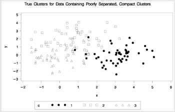
Figure 7.2: Data Containing Poorly Separated, Compact Clusters: Plot of True Clusters

The following statements use the FASTCLUS procedure to find three clusters and the GPLOT procedure to plot the clusters. Since the GPLOT step is repeated several times in this example, it is contained in the PLOTCLUS macro. The following statements produce Figure 7.3.

  %macro plotclus;   legend1 frame cframe=ligr  cborder=black   position=center value=(justify=center);   axis1 minor=none label=(angle=90 rotate=0);   axis2 minor=none;   proc gplot;   plot y*x=cluster/frame cframe=ligr   vaxis=axis1 haxis=axis2 legend=legend1;   run;   %mend plotclus;   proc fastclus data=closer out=out maxc=3 noprint;   var x y;   title 'FASTCLUS Analysis';   title2 'of Data Containing Poorly Separated,   Compact Clusters';   run;   %plotclus;

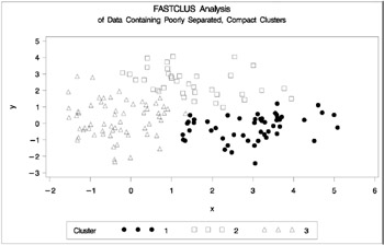
Figure 7.3: Data Containing Poorly Separated, Compact Clusters: PROC FASTCLUS

The following SAS statements produce Figure 7.4:

  proc cluster data=closer outtree=tree method=ward noprint;   var x y;   run;   proc tree noprint out=out n=3;   copy x y;   title 'Ward''s Minimum Variance Cluster Analysis';   title2 'of Data Containing Poorly Separated,   Compact Clusters';   run;   %plotclus;

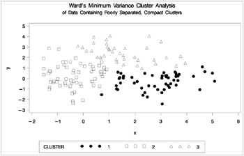
Figure 7.4: Data Containing Poorly Separated, Compact Clusters: PROC CLUSTER with METHOD=WARD

The following SAS statements produce Figure 7.5:

  proc cluster data=closer outtree=tree method=average noprint;   var x y;   run;   proc tree noprint out=out n=3 dock=5;   copy x y;   title 'Average Linkage Cluster Analysis';   title2 'of Data Containing Poorly Separated,   Compact Clusters';   run;   %plotclus;

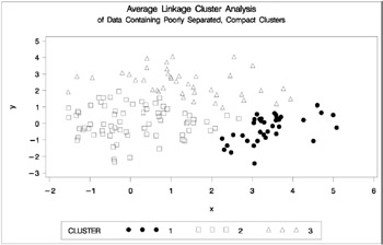
Figure 7.5: Data Containing Poorly Separated, Compact Clusters: PROC CLUSTER with METHOD=AVERAGE

The following SAS statements produce Figure 7.6:

  proc cluster data=closer outtree=tree   method=centroid noprint;   var x y;   run;   proc tree noprint out=out n=3 dock=5;   copy x y;   title 'Centroid Cluster Analysis';   title2 'of Data Containing Poorly Separated,   Compact Clusters';   run;   %plotclus;

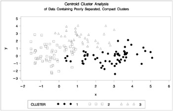
Figure 7.6: Data Containing Poorly Separated, Compact Clusters: PROC CLUSTER with METHOD=CENTROID

The following SAS statements produce Figure 7.7:

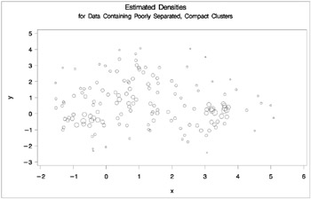
  proc cluster data=closer outtree=tree   method=twostage k=10 noprint;   var x y;   run;   proc tree noprint out=out n=3;   copy x y _dens_;   title 'Two-Stage Density Linkage Cluster Analysis';   title2 'of Data Containing Poorly Separated,   Compact Clusters';   run;   %plotclus;   proc gplot;   bubble y*x=_dens_/frame cframe=ligr   vaxis=axis1 haxis=axis2;   title 'Estimated Densities';   title2 'for Data Containing Poorly Separated,   Compact Clusters';   run;

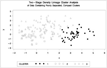
Figure 7.7: Data Containing Poorly Separated, Compact Clusters: PROC CLUSTER with METHOD=TWOSTAGE

In two-stage density linkage, each cluster is a region surrounding a local maximum of the estimated probability density function. If you think of the estimated density function as a landscape with mountains and valleys, each mountain is a cluster, and the boundaries between clusters are placed near the bottoms of the valleys.

The following SAS statements produce Figure 7.8:

  proc cluster data=closer outtree=tree   method=single noprint;   var x y;   run;   proc tree data=tree noprint out=out n=3 dock=5;   copy x y;   title 'Single Linkage Cluster Analysis';   title2 'of Data Containing Poorly Separated,   Compact Clusters';   run;   %plotclus;

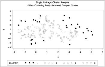
Figure 7.8: Data Containing Poorly Separated, Compact Clusters: PROC CLUSTER with METHOD=SINGLE

The two least-squares methods, PROC FASTCLUS and Ward's, yield the most uniform cluster sizes and the best recovery of the true clusters. This result is expected since these two methods are biased toward recovering compact clusters of equal size. With average linkage, the lower-left cluster is too large; with the centroid method, the lower-right cluster is too large; and with two-stage density linkage, the top cluster is too large. The single linkage analysis resembles average linkage except for the large number of outliers resulting from the DOCK= option in the PROC TREE statement; the outliers are plotted as dots (missing values).

Multinormal Clusters of Unequal Size and Dispersion

In this example, there are three multinormal clusters that differ in size and dispersion. PROC FASTCLUS and five of the hierarchical methods available in PROC CLUSTER are used. To help you compare methods, the true, generated clusters are plotted. The following SAS statements produce Figure 7.9:

  data unequal;   keep x y c;   mx=1; my=0; n=20; scale=.5; c=1; link generate;   mx=6; my=0; n=80; scale=2.; c=3; link generate;   mx=3; my=4; n=40; scale=1.; c=2; link generate;   stop;   generate:   do i=1 to n;   x=rannor(1)*scale+mx;   y=rannor(1)*scale+my;   output;   end;   return;   run;   title 'True Clusters for Data Containing Multinormal   Clusters';   title2 'of Unequal Size';   proc gplot;   plot y*x=c/frame cframe=ligr   vaxis=axis1 haxis=axis2 legend=legend1;   run;

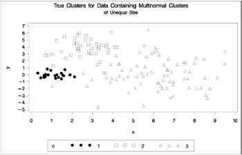
Figure 7.9: Data Containing Generated Clusters of Unequal Size

The following statements use the FASTCLUS procedure to find three clusters and the PLOTCLUS macro to plot the clusters. The statements produce Figure 7.10.

  proc fastclus data=unequal out=out maxc=3 noprint;   var x y;   title 'FASTCLUS Analysis';   title2 'of Data Containing Compact Clusters of   Unequal Size';   run;   %plotclus;

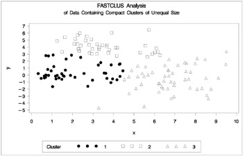
Figure 7.10: Data Containing Compact Clusters of Unequal Size: PROC FASTCLUS

The following SAS statements produce Figure 7.11:

  proc cluster data=unequal outtree=tree   method=ward noprint;   var x y;   run;   proc tree noprint out=out n=3;   copy x y;   title 'Ward''s Minimum Variance Cluster Analysis';   title2 'of Data Containing Compact Clusters of   Unequal Size';   run;   %plotclus;

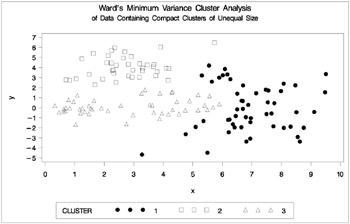
Figure 7.11: Data Containing Compact Clusters of Unequal Size: PROC CLUSTER with METHOD=WARD

The following SAS statements produce Figure 7.12:

  proc cluster data=unequal outtree=tree method=average   noprint;   var x y;   run;   proc tree noprint out=out n=3 dock=5;   copy x y;   title 'Average Linkage Cluster Analysis';   title2 'of Data Containing Compact Clusters of   Unequal Size';   run;   %plotclus;

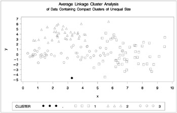
Figure 7.12: Data Containing Compact Clusters of Unequal Size: PROC CLUSTER with METHOD=AVERAGE

The following SAS statements produce Figure 7.13:

  proc cluster data=unequal outtree=tree   method=centroid noprint;   var x y;   run;   proc tree noprint out=out n=3 dock=5;   copy x y;   title 'Centroid Cluster Analysis';   title2 'of Data Containing Compact Clusters of   Unequal Size';   run;   %plotclus;

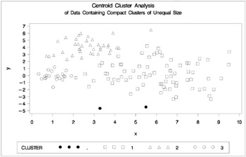
Figure 7.13: Data Containing Compact Clusters of Unequal Size: PROC CLUSTER with METHOD=CENTROID

The following SAS statements produce Figure 7.14:

  proc cluster data=unequal outtree=tree method=twostage   k=10 noprint;   var x y;   run;   proc tree noprint out=out n=3;   copy x y _dens_;   title 'Two-Stage Density Linkage Cluster Analysis';   title2 'of Data Containing Compact Clusters of   Unequal Size';   run;   %plotclus;   proc gplot;   bubble y*x=_dens_/frame cframe=ligr   vaxis=axis1 haxis=axis2 ;   title 'Estimated Densities';   title2 'for Data Containing Compact Clusters of   Unequal Size';   run;

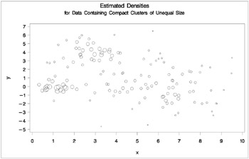
Figure 7.14: Data Containing Compact Clusters of Unequal Size: PROC CLUSTER with METHOD=TWOSTAGE

The following SAS statements produce Figure 7.15:

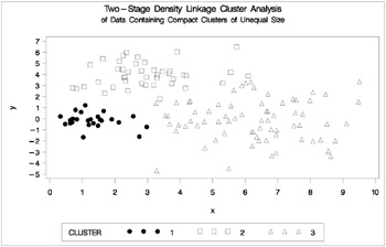
  proc cluster data=unequal outtree=tree   method=single noprint;   var x y;   run;   proc tree data=tree noprint out=out n=3 dock=5;   copy x y;   title 'Single Linkage Cluster Analysis';   title2 'of Data Containing Compact Clusters of   Unequal Size'];   run;   %plotclus;

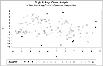
Figure 7.15: Data Containing Compact Clusters of Unequal Size: PROC CLUSTER with METHOD=SINGLE

In the PROC FASTCLUS analysis, the smallest cluster, in the bottom left of the plot, has stolen members from the other two clusters, and the upper-left cluster has also acquired some observations that rightfully belong to the larger, lower-right cluster. With Ward's method, the upper-left cluster is separated correctly, but the lower-left cluster has taken a large bite out of the lower-right cluster. For both of these methods, the clustering errors are in accord with the biases of the methods to produce clusters of equal size. In the average linkage analysis, both the upper- and lower-left clusters have encroached on the lower-right cluster, thereby making the variances more nearly equal than in the true clusters. The centroid method, which lacks the size and dispersion biases of the previous methods, obtains an essentially correct partition.

Two-stage density linkage does almost as well even though the compact shapes of these clusters favor the traditional methods. Single linkage also produces excellent results.

Elongated Multinormal Clusters

In this example, the data are sampled from two highly elongated multinormal distributions with equal covariance matrices. The following SAS statements produce Figure 7.16:

  data elongate;   keep x y;   ma=8; mb=0; link generate;   ma=6; mb=8; link generate;   stop;   generate:   do i=1 to 50;   a=rannor(7)*6+ma;   b=rannor(7)+mb;   x=a-b;   y=a+b;   output;   end;   return;   run;   proc fastclus data=elongate out=out maxc=2 noprint;   run;   proc gplot;   plot y*x=cluster/frame cframe=ligr   vaxis=axis1 haxis=axis2 legend=legend1;   title 'FASTCLUS Analysis';   title2 'of Data Containing Parallel Elongated Clusters';   run;

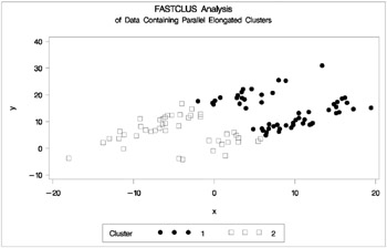
Figure 7.16: Data Containing Parallel Elongated Clusters: PROC FASTCLUS

Notice that PROC FASTCLUS found two clusters, as requested by the MAXC= option. However, it attempted to form spherical clusters, which are obviously inappropriate for this data.

The following SAS statements produce Figure 7.17:

  proc cluster data=elongate outtree=tree   method=average noprint;   run;   proc tree noprint out=out n=2 dock=5;   copy x y;   run;   proc gplot;   plot y*x=cluster/frame cframe=ligr   vaxis=axis1 haxis=axis2 legend=legend1;   title 'Average Linkage Cluster Analysis';   title2 'of Data Containing Parallel Elongated Clusters';   run;

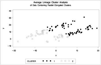
Figure 7.17: Data Containing Parallel Elongated Clusters: PROC CLUSTER with METHOD=AVERAGE

The following SAS statements produce Figure 7.18:

  proc cluster data=elongate outtree=tree   method=twostage k=10 noprint;   run;   proc tree noprint out=out n=2;   copy x y;   run;   proc gplot;   plot y*x=cluster/frame cframe=ligr   vaxis=axis1 haxis=axis2 legend=legend1;   title 'Two-Stage Density Linkage Cluster Analysis';   title2 'of Data Containing Parallel Elongated Clusters';   run;

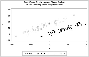
Figure 7.18: Data Containing Parallel Elongated Clusters: PROC CLUSTER with METHOD=TWOSTAGE

PROC FASTCLUS and average linkage fail miserably. Ward's method and the centroid method, not shown, produce almost the same results. Two-stage density linkage, however, recovers the correct clusters. Single linkage, not shown, finds the same clusters as two-stage density linkage except for some outliers.

In this example, the population clusters have equal covariance matrices. If the withincluster covariances are known, the data can be transformed to make the clusters spherical so that any of the clustering methods can find the correct clusters. But when you are doing a cluster analysis, you do not know what the true clusters are, so you cannot calculate the within-cluster covariance matrix. Nevertheless, it is sometimes possible to estimate the within-cluster covariance matrix without knowing the cluster membership or even the number of clusters, using an approach invented by Art, Gnanadesikan, and Kettenring (1982). A method for obtaining such an estimate is available in the ACECLUS procedure.

In the following analysis, PROC ACECLUS transforms the variables X and Y into canonical variables CAN1 and CAN2. The latter are plotted and then used in a cluster analysis by Ward's method. The clusters are then plotted with the original variables X and Y. The following SAS statements produce Figure 7.19:

  proc aceclus data=elongate out=ace p=.1;   var x y;   title 'ACECLUS Analysis';   title2 'of Data Containing Parallel Elongated Clusters';   run;   proc gplot;   plot can2*can1/frame cframe=ligr;   title 'Data Containing Parallel Elongated Clusters';   title2 'After Transformation by PROC ACECLUS';   run;

  ACECLUS Analysis   of Data Containing Parallel Elongated Clusters   The ACECLUS Procedure   Observations         100    Proportion      0.1000   Variables              2    Converge       0.00100   Means and Standard Deviations   Standard   Variable        Mean    Deviation   x             2.6406       8.3494   y            10.6488       6.8420   COV: Total Sample Covariances   x                 y   x       69.71314819       24.24268934   y       24.24268934       46.81324861   Threshold =    0.328478   Iteration History   Pairs   RMS       Distance      Within    Convergence   Iteration    Distance     Cutoff       Cutoff      Measure   ------------------------------------------------------------   1       2.000       0.657       672.0     0.673685   2       9.382       3.082       716.0     0.006963   3       9.339       3.068       760.0     0.008362   4       9.437       3.100       824.0     0.009656   5       9.359       3.074       889.0     0.010269   6       9.267       3.044       955.0     0.011276   7       9.208       3.025       999.0     0.009230   8       9.230       3.032      1052.0     0.011394   9       9.226       3.030      1091.0     0.007924   10       9.173       3.013      1121.0     0.007993   WARNING: Iteration limit exceeded.   ACECLUS Analysis   of Data Containing Parallel Elongated Clusters   The ACECLUS Procedure   ACE: Approximate Covariance Estimate Within Clusters   x                 y   x       9.299329632       8.215362614   y       8.215362614       8.937753936   Eigenvalues of Inv(ACE)*(COV-ACE)   Eigenvalue    Difference    Proportion    Cumulative   1       36.7091       33.1672        0.9120        0.9120   2        3.5420                      0.0880        1.0000   Eigenvectors (Raw Canonical Coefficients)   Can1          Can2   x   .748392      0.109547   y      0.736349      0.230272   Standardized Canonical Coefficients   Can1          Can2   x   6.24866       0.91466   y       5.03812       1.57553

Figure 7.19: Data Containing Parallel Elongated Clusters: PROC ACECLUS

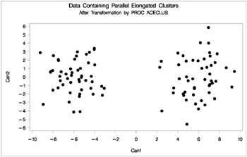
Figure 7.20: Data Containing Parallel Elongated Clusters After Transformation by PROC ACECLUS

The following SAS statements produce Figure 7.21:

  proc cluster data=ace outtree=tree method=ward noprint;   var can1 can2;   copy x y;   run;   proc tree noprint out=out n=2;   copy x y;   run;   proc gplot;   plot y*x=cluster/frame cframe=ligr   vaxis=axis1 haxis=axis2 legend=legend1;   title 'Ward''s Minimum Variance Cluster Analysis';   title2 'of Data Containing Parallel Elongated Clusters';   title3 'After Transformation by PROC ACECLUS';   run;

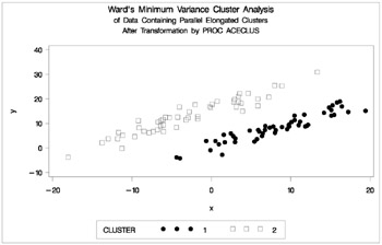
Figure 7.21: Transformed Data Containing Parallel Elongated Clusters: PROC CLUSTER with METHOD=WARD

Nonconvex Clusters

If the population clusters have very different covariance matrices, using PROC ACECLUS is of no avail. Although methods exist for estimating multinormal clusters with unequal covariance matrices (Wolfe 1970; Symons 1981; Everitt and Hand 1981; Titterington, Smith, and Makov 1985; McLachlan and Basford 1988, these methods tend to have serious problems with initialization and may converge to degenerate solutions. For unequal covariance matrices or radically nonnormal distributions, the best approach to cluster analysis is through nonparametric density estimation, as in density linkage. The next example illustrates population clusters with nonconvex density contours . The following SAS statements produce Figure 7.22.

  data noncon;   keep x y;   do i=1 to 100;   a=i*.0628319;   x=cos(a)+(i>50)+rannor(7)*.1;   y=sin(a)+(i>50)*.3+rannor(7)*.1;   output;   end;   run;   proc fastclus data=noncon out=out maxc=2 noprint;   run;   proc gplot;   plot y*x=cluster/frame cframe=ligr   vaxis=axis1 haxis=axis2 legend=legend1;   title 'FASTCLUS Analysis';   title2 'of Data Containing Nonconvex Clusters';   run;

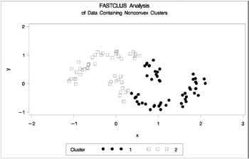
Figure 7.22: Data Containing Nonconvex Clusters: PROC FASTCLUS

The following SAS statements produce Figure 7.23.

  proc cluster data=noncon outtree=tree   method=centroid noprint;   run;   proc tree noprint out=out n=2 dock=5;   copy x y;   run;   proc gplot;   plot y*x=cluster/frame cframe=ligr   vaxis=axis1 haxis=axis2 legend=legend1;   title 'Centroid Cluster Analysis';   title2 'of Data Containing Nonconvex Clusters';   run;

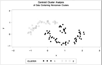
Figure 7.23: Data Containing Nonconvex Clusters: PROC CLUSTER with METHOD=CENTROID

The following SAS statements produce Figure 7.24.

  proc cluster data=noncon outtree=tree   method=twostage k=10 noprint;   run;   proc tree noprint out=out n=2;   copy x y;   run;   proc gplot;   plot y*x=cluster/frame cframe=ligr   vaxis=axis1 haxis=axis2 legend=legend1;   title 'Two-Stage Density Linkage Cluster Analysis';   title2 'of Data Containing Nonconvex Clusters';   run;

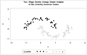
Figure 7.24: Data Containing Nonconvex Clusters: PROC CLUSTER with METHOD=TWOSTAGE

Ward's method and average linkage, not shown, do better than PROC FASTCLUS but not as well as the centroid method. Two-stage density linkage recovers the correct clusters, as does single linkage, which is not shown.

The preceding examples are intended merely to illustrate some of the properties of clustering methods in common use. If you intend to perform a cluster analysis, you should consult more systematic and rigorous studies of the properties of clustering methods, such as Milligan (1980).