22.3 Constraint-Based Typing

< Free Open Study >

We now present an algorithm that, given a term t and a context Г, calculates a set of constraints-equations between type expressions (possibly involving type variables)-that must be satisfied by any solution for (Г, t). The intuition behind this algorithm is essentially the same as the ordinary typechecking algorithm; the only difference is that, instead of checking constraints, it simply records them for later consideration. For example, when presented with an application t₁ t₂ with Г ⊢ t₁ : T₁ and Г ⊢ t₂ : T₂, rather than checking that t₁ has the form T₂→T₁₂ and returning T₁₂ as the type of the application, it instead chooses a fresh type variable X, records the constraint T₁ = T₂→X, and returns X as the type of the application.

22.3.1 Definition

A constraint set C is a set of equations {S_i = T_i^{iÎ 1..n}}. A substitution σ is said to unify an equation S = T if the substitution instances σS and σT are identical. We say that σ unifies (or satisfies) C if it unifies every equation in C.

22.3.2 Definition

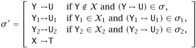
The constraint typing relation Г ⊢ t : T |_x C is defined by the rules in Figure 22-1. Informally, Г ⊢ t : T |_x C can be read "term t has type T under assumptions Г whenever constraints C are satisfied." In rule T-APP, we write FV(T) for the set of all type variables mentioned in T.

The X subscripts are used to track the type variables introduced in each subderivation and make sure that the fresh variables created in different subderivations are actually distinct. On a first reading of the rules, it may be helpful to ignore these subscripts and all the premises involving them. On the next reading, observe that these annotations and premises ensure two things. First, whenever a type variable is chosen by the final rule in some derivation, it must be different from any variables chosen in subderivations. Second, whenever a rule involves two or more subderivations, the sets of variables chosen by these subderivations must be disjoint. Also, note that these conditions never prevent us from building some derivation for a given term; they merely prevent us from building a derivation in which the same variable is used "fresh" in two different places. Since there is an infinite supply of type variable names, we can always find a way of satisfying the freshness requirements.

When read from bottom to top, the constraint typing rules determine a straightforward procedure that, given Г and t, calculates T and C (and X) such that Г ⊢ t : T |_x C. However, unlike the ordinary typing algorithm for the simply typed lambda-calculus, this one never fails, in the sense that for every Г and t there are always some T and C such that Г ⊢ t : T |_x C, and moreover that T and C are uniquely determined by Г and t. (Strictly speaking, the algorithm is deterministic only if we consider it "modulo the choice of fresh names." We return to this point in Exercise 22.3.9.)

To lighten the notation in the following discussion, we sometimes elide the X and write just Г ⊢ t : T | C.

22.3.3 Exercise [⋆ ↛]

Construct a constraint typing derivation whose conclusion is

   ⊢ λx:X. λy:Y. λz:Z. (x z) (y z) : S |_x C

for some S, X, and C.

The idea of the constraint typing relation is that, given a term t and a context Г, we can check whether t is typable under Г by first collecting the constraints C that must be satisfied in order for t to have a type, together with a result type S, sharing variables with C, that characterizes the possible types of t in terms of these variables. Then, to find solutions for t, we just look for substitutions σ that satisfy C (i.e., that make all the equations in C into identities); for each such σ, the type σS is a possible type of t. If we find that there are no substitutions that satisfy C, then we know that t cannot be instantiated in such a way as to make it typable.

For example, the constraint set generated by the algorithm for the term t = λx:X→Y. x 0 is {Nat→Z = X→Y}, and the associated result type is (X→Y)→Z.The substitution σ = [X ↦ Nat, Z ↦ Bool, Y ↦ Bool] makes the equation Nat→Z = X→Y into an identity, so we know that σ((X→Y)→Z), i.e., (Nat→Bool)→Bool, is a possible type for t.

This idea is captured formally by the following definition.

22.3.4 Definition

Suppose that Г ⊢ t : S |C. A solution for (Г, t, S, C) is a pair (σ, T) such that σ satisfies C and σS = T.

The algorithmic problem of finding substitutions unifying a given constraint set C will be taken up in the next section. First, though, we should check that our constraint typing algorithm corresponds in a suitable sense to the original, declarative typing relation.

Given a context Г and a term t, we have two different ways of characterizing the possible ways of instantiating type variables in Г and t to produce a valid typing:

[DECLARATIVE] as the set of all solutions for (Г, t) in the sense of Definition 22.2.1; or
[ALGORITHMIC] via the constraint typing relation, by finding S and C such that Г ⊢ t : S | C and then taking the set of solutions for (Г, t, S, C).

We show the equivalence of these two characterizations in two steps. First we show that every solution for (Г, t, S, C) is also a solution for (Г, t) (Theorem 22.3.5). Then we show that every solution for (Г, t) can be extended to a solution for (Г, t, S, C) (Theorem 22.3.7) by giving values for the type variables introduced by constraint generation.

22.3.5 Theorem [Soundness of Constraint Typing]

Suppose that Г ⊢ t : S | C. If (σ, T) is a solution for (Г, t, S, C), then it is also a solution for (Г, t).

For this direction of the argument, the fresh variable sets X are secondary and can be elided.

Proof: By induction on the given constraint typing derivation for Г ⊢ t : S | C, reasoning by cases on the last rule used.

Case CT-VAR:

t = x

x:S Î Г

C = {}

We are given that (σ, T) is a solution for (Г, t, S, C); since C is empty, this means just that σS = T. But then by T-VAR we immediately obtain σГ ⊢ x : T, as required.

Case CT-ABS:

t = λx:T₁ .t₂

S = T₁→S₂

Г, x:T₁ ⊢ t₂ : S₂ | C

We are given that (σ, T) is a solution for (Г, t, S, C), that is, σ unifies C and T = σS = σT₁ → σS₂. So (σ, σS₂) is a solution for (Г, t₂, S₂, C). By the induction hypothesis, (σ, σS₂) is a solution for ((Г, x:T₁), t₂), i.e., σГ, x:σT₁ ⊢ σ t₂ : σS₂. By T-ABS, σГ ⊢ λx:σT₁.σt₂ : σT₁ → σS₂ = σ(T₁→S₂) = T, as required.

Case CT-APP:	t = t₁ t₂	S = X
	Г ⊢ t₁ : S₁ \| C₁	Г ⊢ t₂ : S₂ \| C₂
	C = C₁ È C₂ È {S₁ = S₂→X}

By definition, σ unifies C₁ and C₂ and σS₁ = σ(S₂→X). So (σ, σS₁) and (σ, σS₂) are solutions for (Г, t₁, S₁, C₁) and (Г, t₂, S₂, C₂), from which the induction hypothesis gives us σГ ⊢ σt₁ : σS₁ and σГ ⊢ sgrt₂ : σS₂. But since σS₁ = σS₂→σX, we have σГ ⊢ σt₁ : σS₂→σX, and, by T-APP, σГ ⊢ σ(t₁ t₂) : σX = T.

Other cases:

Similar.

The argument for the completeness of constraint typing with respect to the ordinary typing relation is a bit more delicate, because we must deal carefully with fresh names.

22.3.6 Definition

Write σ\X for the substitution that is undefined for all the variables in X and otherwise behaves like σ.

22.3.7 Theorem [Completeness of Constraint Typing]

Suppose Г ⊢ t : S |_x C. If (σ, T) is a solution for (Г, t) and dom(σ) ∩ X = , then there is some solution (σ′, T) for (Г, t,S, C) such that σ′\X = σ.

Proof: By induction on the given constraint typing derivation.

Case CT-VAR:

t = x

x:S Î Г

From the assumption that (σ, T) is a solution for (Г, x), the inversion lemma for the typing relation (9.3.1) tells us that T = σS. But then (σ, T) is also a (Г, x,S, {})-solution.

Case CT-ABS:

t = λx:T₁ . t₂

Г, x: T₁ ⊢ t₂ : S₂ |_x C

S = T₁→S₂

From the assumption that (σ, T) is a solution for (Г, λx:T₁ .t₂), the inversion lemma for the typing relation yields σГ, x:σT₁ ⊢ σt₂ : T₂ and T = σT₁→T₂ for some T₂. By the induction hypothesis, there is a solution (σ′, T₂) for ((Г,x:T₁), t₂, S₂, C) such that σ′\X agrees with σ. Now, X cannot include any of the type variables in T₁. So σ′T₁ = σT₁, and σ′(S) = σ′(T₁→S₂) = σT₁→σ′S₂ = σT₁→T₂ = T. Thus, we see that (σ′, T) is a solution for (Г, (λx:T₁ .t₂), T₁→S₂, C).

Case CT-APP:	t = t₁ t₂	Г ⊢ t₁ :S₁ C₁	Г ⊢′t₂ :S₂ C₂
	X₁ ∩ X₂ = 
	X₁ ∩ FV(T₂) = 
	X₂ ∩ FV(T₁) = 
	X not mentioned in X₁, X₂, S₁, S₂, C₁ C₂
	S = X	X = X₁ È X₂ È {X}	C = C₁ ∩ C₂ ∩ {S₁ = S₂→X}

From the assumption that (σ, T) is a solution for (Г, t₁ t₂), the inversion lemma for the typing relation yields σГ ⊢ σt₁ : T₁T and σГ ⊢ σt₂ : T₁. By the induction hypothesis, there are solutions (σ₁, T₁→T) for (Г, t₁, S₁, C₁) and (σ₂, T₁) for (Г, t₂, S₂, C₂), and σ₁\X₁ = σ = σ₂\X₂. We must exhibit a substitution σ′ such that: (1) σ′\X agrees with σ; (2) σ′X = T; (3) σ′ unifies C₁ and C₂; and (4) σ′ unifies {S₁ = S₂→X}, i.e., σ′S₁ = σ′S₂→ σ′X. Define σ′ as follows:

Conditions (1) and (2) are obviously satisfied. (3) is satisfied because X₁ and X₂ do not overlap. To check (4), first note that the side-conditions about freshness guarantee that FV(S₁) ∩ (X₂ È {X}) = , so that σ′S₁ = σ₁S₁. Now calculate as follows: σ′S₁ = σ₁S₁ = T₁→T = σ₂S₂→T = σ′ S₂→σ′X = σ′ (S₂→X).

Other cases:

Similar.

22.3.8 Corollary

Suppose Г ⊢ t : S | C. There is some solution for (Г, t) iff there is some solution for (Г, t, S, C).

Proof: By Theorems 22.3.5 and 22.3.7.

22.3.9 Exercise [Recommended, ⋆⋆⋆]

In a production compiler, the nondeterministic choice of a fresh type variable name in the rule CT-APP would typically be replaced by a call to a function that generates a new type variable-different from all others that it ever generates, and from all type variables mentioned explicitly in the context or term being checked-each time it is called. Because such global "gensym" operations work by side effects on a hidden global variable, they are difficult to reason about formally. However, we can mimic their behavior in a fairly accurate and mathematically more tractable way by "threading" a sequence of unused variable names through the constraint generation rules.

Let F denote a sequence of distinct type variable names. Then, instead of writing Г ⊢ t : T |_x C for the constraint generation relation, we write Г⊢_F t : T |_F′ C, where Г, F, and t are inputs to the algorithm and T, F′, and C are outputs. Whenever it needs a fresh type variable, the algorithm takes the front element of F and returns the rest of F as F′.

Write out the rules for this algorithm. Prove that they are equivalent, in an appropriate sense, to the original constraint generation rules.

22.3.10 Exercise [Recommended, ⋆⋆]

Implement the algorithm from Exercise 22.3.9 in ML. Use the datatype

   type ty =       TyBool     | TyArr of ty * ty     | TyId of string     | TyNat

for types, and

   type constr = (ty * ty) list

for constraint sets. You will also need a representation for infinite sequences of fresh variable names. There are lots of ways of doing this; here is a fairly direct one using a recursive datatype:

   type nextuvar = NextUVar of string * uvargenerator   and uvargenerator = unit → nextuvar   let uvargen =     let rec f n () = NextUVar("?X_" ∧ string_of_int n, f (n+1))     in f 0

That is, uvargen is a function that, when called with argument (), returns a value of the form NextUVar(x,f), where x is a fresh type variable name and f is another function of the same form.

22.3.11 Exercise [⋆⋆]

Show how to extend the constraint generation algorithm to deal with general recursive function definitions (§11.11).

< Free Open Study >