22.4 Unification

< Free Open Study >

To calculate solutions to constraint sets, we use the idea, due to Hindley (1969) and Milner (1978), of using unification (Robinson, 1971) to check that the set of solutions is nonempty and, if so, to find a "best" element, in the sense that all solutions can be generated straightforwardly from this one.

22.4.1 Definition

A substitution σ is less specific (or more general) than a substitution σ′, written σ ⊑ σ′, if σ′ = γ ∘ σ for some substitution γ.

22.4.2 Definition

A principal unifier (or sometimes most general unifier) for a constraint set C is a substitution σ that satisfies C and such that σ ⊑ σ′ for every substitution σ′ satisfying C.

22.4.3 Exercise [⋆]

Write down principal unifiers (when they exist) for the following sets of constraints:

    {X = Nat, Y = X→X}      {Nat→Nat = X→Y}    {X→Y = Y→Z, Z = U→W}    {Nat = Nat→Y}    {Y = Nat→Y}             {}  (the empty set of constraints)

22.4.4 Definition

The unification algorithm for types is defined in Figure 22-2.^[3] The phrase "let {S = T} ÈC′ = C" in the second line should be read as "choose a constraint S=T from the set C and let C′ denote the remaining constraints from C.

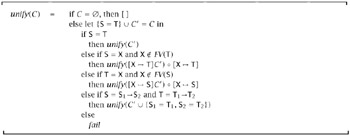
Figure 22-2: Unification Algorithm

The side conditions X ∉ FV(T) in the fifth line and X ∉ FV(S) in the seventh are known as the occur check. Their effect is to prevent the algorithm from generating a solution involving a cyclic substitution like X ↦ X→X, which makes no sense if we are talking about finite type expressions. (If we expand our language to include infinite type expressions-i.e. recursive types in the sense of Chapters 20 and 21-then the occur check can be omitted.)

22.4.5 Theorem

The algorithm unify always terminates, failing when given a non-unifiable constraint set as input and otherwise returning a principal unifier. More formally:

unify(C) halts, either by failing or by returning a substitution, for all C;
if unify(C) = σ, then σ is a unifier for C;
if δ is a unifier for C, then unify(C) = σ with σ ⊑ δ.

Proof: For part (1), define the degree of a constraint set C to be the pair (m, n), where m is the number of distinct type variables in C and n is the total size of the types in C. It is easy to check that each clause of the unify algorithm either terminates immediately (with success in the first case or failure in the last) or else makes a recursive call to unify with a constraint set of lexicographically smaller degree.

Part (2) is a straightforward induction on the number of recursive calls in the computation of unify(C). All the cases are trivial except for the two involving variables, which depend on the observation that, if σ unifies [X ↦ T]D, then σ ∘ [X ↦ T] unifies {X = T} È D for any constraint set D.

Part (3) again proceeds by induction on the number of recursive calls in the computation of unify(C). If C is empty, then unify(C) immediately returns the trivial substitution [ ]; since δ = δ ∘ [ ], we have [ ] ⊑ δ as required. If C is non-empty, then unify(C) chooses some pair (S, T) from C and continues by cases on the shapes of S and T.

Case:

S = T

Since δ is a unifier for C, it also unifies C′. By the induction hypothesis, unify(C) = σ with σ ⊑ δ, as required.

Case:

S = X and X ∉ FV(T)

Since δ unifies S and T, we have δ(X) = δ(T). So, for any type U, we have δ(U) = δ([X ↦ T]U) in particular, since δ unifies C′, it must also unify [X ↦ T]C′. The induction hypothesis then tells us that unify([X ↦ T]C′) = σ′, with δ = γ ∘ σ′ for some γ. Since unify(C) = σ′ ∘ [X ↦ T], showing that δ = γ ∘ (σ′ ∘ [X ↦ T]) will complete the argument. So consider any type variable Y. If Y ≠ X, then clearly (γ ∘ (σ′ ∘ [X ↦ T]))Y = (γ ∘ σ′)Y = δY. On the other hand, (γ ∘ (σ′ ∘ [X ↦ T]))X = (γ ∘ σ′)T = δX, as we saw above. Combining these observations, we see that δY = (γ ∘ (σ′ ∘ [X ↦ T]))Y for all variables Y, that is, δ = (γ ∘ (σ′ ∘ [X ↦ T])).

Case:

T = X and X ∉ FV(S)

Similar.

Case:

S = S₁→S₂ and T = T₁→T₂

Straightforward. Just note that δ is a unifier of {S₁→S₂ = T₁→T₂} È C′ iff it is a unifier of C′ È {S₁ = T₁, S₂ = T₂}.

If none of the above cases apply to S and T, then unify(C) fails. But this can happen in only two ways: either S is Nat and T is an arrow type (or vice versa), or else S = X and X Î T (or vice versa). The first case obviously contradicts the assumption that C is unifiable. To see that the second does too, recall that, by assumption, δS = δT; if X occurred in T, then δT would always be strictly larger than δSS. Thus, if unify(C) fails, then C is not unifiable, contradicting our assumption that δ is a unifier for C; so this case cannot occur.

22.4.6 Exercise [Recommended, ⋆⋆⋆]

Implement the unification algorithm.

^[3]Note that nothing in this algorithm depends on the fact that we are unifying type expressions as opposed to some other sort of expressions; the same algorithm can be used to solve equality constraints between any kind of (first-order) expressions.

< Free Open Study >