Section 4.5. Polynomial Arithmetic
4.5. Polynomial ArithmeticBefore pursuing our discussion of finite fields, we need to introduce the interesting subject of polynomial arithmetic. We are concerned with polynomials in a single variable x, and we can distinguish three classes of polynomial arithmetic:
This section examines the first two classes, and the next section covers the last class. Ordinary Polynomial ArithmeticA polynomial of degree n (integer n where the ai are elements of some designated set of numbers S, called the coefficient set, and an In the context of abstract algebra, we are usually not interested in evaluating a polynomial for a particular value of x [e.g., f(7)]. To emphasize this point, the variable x is sometimes referred to as the indeterminate. Polynomial arithmetic includes the operations of addition, subtraction, and multiplication. These operations are defined in a natural way as though the variable x was an element of S. Division is similarly defined, but requires that S be a field. Examples of fields include the real numbers, rational numbers, and Zp for p prime. Note that the set of all integers is not a field and does not support polynomial division. Addition and subtraction are performed by adding or subtracting corresponding coefficients. Thus, if then addition is defined as and multiplication is defined as where ck = a0bk1 + a1bk1 + ... + ak1b1 + akb0 In the last formula, we treat ai as zero for i > n and bi as zero for i > m. Note that the degree of the product is equal to the sum of the degrees of the two polynomials.
Polynomial Arithmetic with Coefficients in ZpLet us now consider polynomials in which the coefficients are elements of some field F. We refer to this as a polynomial over the field F. In that case, it is easy to show that the set of such polynomials is a ring, referred to as a polynomial ring. That is, if we consider each distinct polynomial to be an element of the set, then that set is a ring.[5]
When polynomial arithmetic is performed on polynomials over a field, then division is possible. Note that this does not mean that exact division is possible. Let us clarify this distinction. Within a field, given two elements a and b, the quotient a/b is also an element of the field. However, given a ring R that is not a field, in general division will result in both a quotient and a remainder; this is not exact division.
Now, if we attempt to perform polynomial division over a coefficient set that is not a field, we find that division is not always defined.
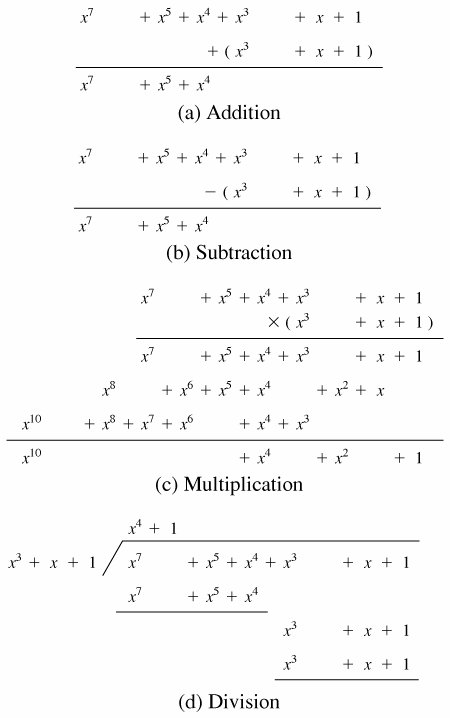
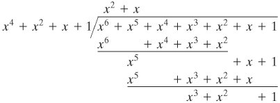
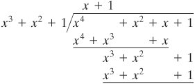
However, as we demonstrate presently, even if the coefficient set is a field, polynomial division is not necessarily exact. In general, division will produce a quotient and a remainder: Equation 4-6 If the degree of f(x) is n and the degree of g(x) is m, (m In an analogy to integer arithmetic, we can write f(x) mod g(x) for the remainder r(x) in Equation (4.6). That is, r(x) = f(x) mod g(x). If there is no remainder [i.e., r(x) = 0 ], then we can say g(x) divides f(x), written as g(x)|f(x); equivalently, we can say that g(x) is a factor of f(x) or g(x) is a divisor of f(x).
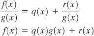
For our purposes, polynomials over GF(2) are of most interest. Recall from Section 4.4 that in GF(2), addition is equivalent to the XOR operation, and multiplication is equivalent to the logical AND operation. Further, addition and subtraction are equivalent mod 2: 1 + 1 = 1 1 = 0; 1 + 0 = 1 0 = 1; 0 + 1 = 0 1 = 1.
A polynomial f(x) over a field F is called irreducible if and only if f(x) cannot be expressed as a product of two polynomials, both over F, and both of degree lower than that of f(x). By analogy to integers, an irreducible polynomial is also called a prime polynomial.
Finding the Greatest Common DivisorWe can extend the analogy between polynomial arithmetic over a field and integer arithmetic by defining the greatest common divisor as follows. The polynomial c(x) is said to be the greatest common divisor of a(x) and b(x) if
An equivalent definition is the following: gcd[a(x), b(x)] is the polynomial of maximum degree that divides both a(x) and b(x). We can adapt the Euclidean algorithm to compute the greatest common divisor of two polynomials. The equality in Equation (4.4) can be rewritten as the following theorem: Equation 4-7 The Euclidean algorithm for polynomials can be stated as follows. The algorithm assumes that the degree of a(x) is greater than the degree of b(x). Then, to find gcd[a(x), b(x)], EUCLID[a(x), b(x)] 1. A(x)
SummaryWe began this section with a discussion of arithmetic with ordinary polynomials. In ordinary polynomial arithmetic, the variable is not evaluated; that is, we do not plug a value in for the variable of the polynomials. Instead, arithmetic operations are performed on polynomials (addition, subtraction, multiplication, division) using the ordinary rules of algebra. Polynomial division is not allowed unless the coefficients are elements of a field. Next, we discussed polynomial arithmetic in which the coefficients are elements of GF(p). In this case, polynomial addition, subtraction, multiplication, and division are allowed. However, division is not exact; that is, in general division results in a quotient and a remainder. Finally, we showed that the Euclidean algorithm can be extended to find the greatest common divisor of two polynomials whose coefficients are elements of a field. All of the material in this section provides a foundation for the following section, in which polynomials are used to define finite fields of order pn. |
 0) is an expression of the form
 0. We say that such polynomials are defined over the coefficient set
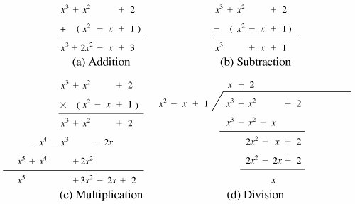


EAN: 2147483647
Pages: 209