Working with Comparison Predicates and Grouped Queries

Understanding Comparison Predicates

An SQL predicate is an expression (often referred to as search condition) in a WHERE clause that asserts a fact. If the assertion is TRUE for a given row in a table, the DBMS performs the action specified by the SQL statement; if the assertion is FALSE, the DBMS goes on to check the predicate against the column values in the next row of the input table. In short, a predicate acts as a filter, allowing only rows that meet its specifications to pass through for further processing.

Table 256.1 shows the six comparison operators you can use to write a comparison predicate.

Table 256.1: SQL Comparison Operators

Operator	Usage	Meaning
=	A = B	Process when A is equal to B
<	A < B	Process when A is less than B
<=	A <= B	Process when A is less than or equal to B
>	A > B	Process when A is greater than "B"
>=	A >= B	Process when A is greater than or equal to B
<>	A <> B	Process when A is not equal to B

Although you can use a comparison operator to compare any two values-even two literals (constants)-the true value of a comparison predicate is that it lets you identify rows you want based on the value stored in each of one or more columns. For example, the comparison predicate in the WHERE clause of the statement

 SELECT * FROM customers WHERE 5 = 5

is of no use as a filter, since 5 is equal to 5 for all rows in the table. As such, the query will display every row in the EMPLOYEE table and could have been written more efficiently without the WHERE clause as:

 SELECT * FROM customers

Conversely, the statement

 DELETE FROM invoices WHERE invoice_date < '01/01/1900'

tells the DBMS to remove only those rows for invoices dated prior to 01/01/1900 from the INVOICES table. Similarly the comparison predicate in the statement

 SELECT cust_ID, cust_name, last_paid, amt_paid, still_due
 FROM customers
 WHERE (GETDATE() - last_paid) > 30
 AND total_due > 500

tells the DBMS to display only those customers who have outstanding balances greater than $500 and who have not made a payment within the last 30 days. Finally, the UPDATE statement

 UPDATE customers
 SET salesperson = 'Konrad' WHERE salesperson = 'Kris'

tells the DBMS to change the value in the SALESPERSON column to Konrad only in those rows that currently have Kris as the SALESPERSON.

Note 

Each comparison operator always works with two values. However, you can test for as many column values as you like (two at a time) by joining multiple comparison predicates using the Boolean operators (OR, AND, and NOT) that you learned about in Tip 94, "Using Boolean Operators OR, AND, and NOT in a WHERE Clause."

Using the BETWEEN Keyword in a WHERE Clause to Select Rows

When you want to work with a set of rows with a column value that lies within a specified range of values, use the keyword BETWEEN in the statement's WHERE clause. For example, to get a list of employees hired during the month of March 2000, you can use a SELECT statement similar to that shown in the MS-SQL Server Query Analyzer input pane near the top of Figure 257.1 to produce a results table similar to that shown at the bottom of the figure.

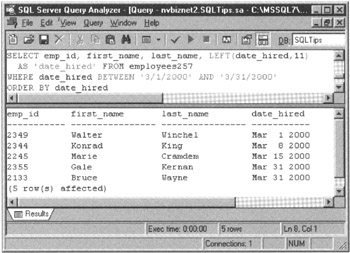
Figure 257.1: MS-SQL Server Query Analyzer query and results table using the BETWEEN keyword

Although the SELECT statement in the current example shows a query in which the upper and lower bounds of the range are literal values, the BETWEEN predicate can actually consist of any three valid SQL expressions with compatible data types, using the syntax:

 
 BETWEEN  AND 

For example, you can use the SELECT statement

 SELECT * FROM employees
 WHERE (total_sales - 25000)
 BETWEEN (SELECT AVG(total_sales) FROM employees)
 AND (SELECT AVG(total_sales) * 1.2 FROM employees)

to list those employees whose total sales volume minus $25,000, is between the average sales volume and 120 percent of the average.

The BETWEEN predicate evaluates to TRUE whenever the value of is greater than or equal to the value of and less than or equal to the value of . Therefore, the query

 SELECT first_name, last_name FROM employees
 WHERE last_name BETWEEN 'J' and 'Qz'

is equivalent to:

 SELECT first_name, last_name FROM employees
 WHERE last_name >= 'J' and last_name <= 'Qz'

One thing to keep in mind is that the value of the low end of the range () must be less than or equal to the value of the high end of the range (). While query

SELECT * FROM employees WHERE date_hired
BETWEEN '01/01/2000' AND '01/31/2000'

may appear to be equivalent to

 SELECT * FROM employees WHERE date_hired
 BETWEEN '01/31/2000' AND '01/01/2000'

it is not. The first query lists employees hired in January 2000, while the second query will never list any employees because it can never be the case that the DATE_HIRED is greater than or equal to 01/31/2000 (the ) while at the same time being less than or equal to 01/01/2000 (the ).

Using the IN or NOT IN Predicate in a WHERE Clause to Select Rows

IN and NOT IN predicates let you select a row based on whether or not the row has a column value that is a member of (included in) a set of values. Suppose, for example, that your company has offices in Nevada, California, Utah, and Texas. Since you have to collect sales tax for customers living in those states, you could use the IN predicate in an UPDATE statement such as

 UPDATE invoices SET sales_tax = invoice_total * 0.07
 WHERE ship_to_state IN ('NV', 'CA', 'UT', 'TX')

to compute the sales tax (given that each state charges the same 7 percent sales tax rate). Conversely, the NOT IN predicate in an UPDATE statement such as

 UPDATE invoices SET sales_tax = 0.00
 WHERE ship_to_state NOT IN ('NV', 'CA', 'UT', 'TX')

will set sales tax due to 0.00 for customers that do not live any of the states in which your company has offices.

The syntax for the IN and NOT IN predicates is:

 [NOT] IN ( [...,.])

While the IN predicate evaluates to TRUE if the is a member of the set of values listed between the parenthesis ( () ), the NOT IN predicate evaluates to TRUE if the is not a member of the set.

As was the case with the BETWEEN predicate (which you learned about in Tip 257, "Using the BETWEEN Keyword in a WHERE Clause to Select Rows"), the IN and NOT IN predicates do not really add to the expressive power of SQL. In the current example, you could have written the UPDATE statement by testing for multiple equalities (joined with OR operators) such as:

 UPDATE invoices SET sales_tax = invoice_total * 0.07
 WHERE ship_to_state = 'NV' OR ship_to_state = 'CA' OR
 ship_to_state = 'UT' OR ship_to_state = 'TX'

However, the IN (and NOT IN) predicate does save you some typing if there are a large number of values in the set you are testing for membership (or exclusion) of the value of the .

Using Wildcard Characters in the LIKE Predicate

You can use the LIKE predicate to query the database for a character string value when you know only a portion of the string you want. As such, the keyword LIKE when used in a WHERE clause lets you compare two character strings for a partial match and is especially valuable when you have some idea of the string's contents but do not know its exact form.

The LIKE predicate has two wildcard characters you can use to write the search string when you know only its general form and not all of its characters. The percent sign (%) can stand for any string of zero or more characters in length, and underscore (_) can stand for any single character. To search for a character string using one or more wildcard characters in a LIKE query, simply include the wildcard(s) in a string literal along with the portion of the string you know.

For example, to search for all teachers whose last names begin with the letters "Ki," you could execute a SELECT statement similar to

 SELECT first_name, last_name FROM faculty
 WHERE last_name LIKE 'Ki%'

which will produce a results table similar to:

first_name last_name
---------- ---------
Konrad King
Wally Kingsly
Sam Kingston

Each of the rows selected from the FACULTY table has a LAST_NAME value staring with the two letters "Ki" and followed by any number of other characters.

Similarly, if you want to match any single character vs. any multiple characters, you would use the underscore (_) instead of the percent sign (%). For example, if you know that the letter S was the second character of any class in the Sciences curriculum, and you wanted a list of 100-level courses, you could execute a SELECT statement similar to

SELECT course_ID, description FROM curriculum
WHERE course_ID LIKE '_S10_'

to produce a results table similar to:

 course_ID description
 --------- -----------------------------------------
 CS101 Introduction to Computer Science
 BS109 Biological Sciences - Anatomy & Physiology
 MS107 Beginning Quadratic Equations

Each of the rows the DBMS selects from the CURRICULUM table has COURSE_ID value with S as the second character, followed by 10, and ending with one and only one additional character. Unlike the percent sign (%) wildcard, which can match zero or more characters, the underscore (_) wildcard can match one and only one character. As such, in the current example, the course_IDs S101 and CS101H would not be included in the query's results table. The S in S101 is the first and not the second character, and two characters instead of one follow the 10 in CS101H.

Using Escape Characters in the LIKE Predicate

In Tip 259, "Using Wildcard Characters in the LIKE Predicate," you learned how to use wildcard characters in a LIKE predicate to query the database for string values when you know only a portion of the string you want. However, what do you do when you want to search for a string that includes one of the wildcard characters?

To check for the existence of a percent sign (%) in a character data type column, for example, you need a way to tell the DBMS to treat a percent sign (%) in the LIKE predicate as a literal value instead of a wildcard. The keyword ESCAPE lets you identify a character that tells the DBMS to treat the character immediately following the escape character in the search string as a literal value. For example, the query

 SELECT cust_ID, cust_name, discount FROM customers
 WHERE discount LIKE "%S%" ESCAPE 'S'

uses the escape character S to tell the DBMS to treat the second percent sign (%) in the search string %S% as a literal value (and not a wildcard). As a result, the query will return the CUST_ID, CUST_NAME, and DISCOUNT column values for any rows in which the last character in the DISCOUNT column is a percent sign (%).

Similarly, if you want to search for the underscore (_) character in a data type column, you would use the keyword ESCAPE in a query such as

 SELECT product_code, description FROM inventory
 WHERE product_code LIKE "XY$_%" ESCAPE '$'

to tell the DBMS to treat the character following the dollar sign ($) as a literal character instead of a wildcard. As a result, of the query in the current example, the DBMS will display the PRODUCT_CODE and DESCRIPTION of all INVENTORY items in which the product code starts with "XY_".

Using LIKE and NOT LIKE to Compare Two Character Strings

SQL has two predicates that let you search the contents of a CHARACTER, VARCHAR, or TEXT data type column for a pattern of characters. The LIKE predicate will return the set of rows in which the target column contains the pattern of characters in the search string. Conversely, the NOT LIKE predicate will return those rows in which the pattern is not found in the target column.

For example, the query

 SELECT * FROM customers WHERE cust_name LIKE 'KING'

will display rows in the CUSTOMERS table in which the value in the target column (CUST_NAME) is KING. Meanwhile, the query

 SELECT * FROM customers WHERE cust_name NOT LIKE 'SMITH'

will display the rows in the CUSTOMERS table that do not have SMITH in the CUST_NAME column.

The LIKE and NOT LIKE predicates are of little value if not used with the wildcard characters you learned about in Tip 259, "Using Wildcard Characters in the LIKE Predicate." After all, you could have written the two example queries using the equality (=) and not equal to (<>) comparison operators, as follows:

 SELECT * FROM customers WHERE cust_name = 'KING'
 SELECT * FROM customers WHERE cust_name <> 'SMITH'

In short, the LIKE predicate is useful when you "know" only some of the characters in the target column, or if you want to work with all rows that contain a certain pattern of characters. For example, if you "know" the name of the customer is something like KING, but you are not sure if it is KINGSLY, KING, or KINGSTON, you could query the database using a SELECT statement similar to:

 SELECT * FROM customers WHERE cust_name LIKE 'KING%'

The percent sign (%) wildcard character tells the DBMS to match any zero of more characters. As such, the query in the current example tells the DBMS to display the columns in a CUSTOMERS table rows in which the value of the target column (CUST_NAME) starts with the letters KING followed by any zero or more additional characters.

Similarly, if you precede the search string with a percent sign (%) you can search for a pattern of characters within a string. For example, the query

SELECT * FROM customers WHERE notes LIKE "%give%discount%"

will display the rows in the CUSTOMERS table in which the value in the target column (NOTES) includes the word GIVE followed by at least one occurrence of the word DISCOUNT. Therefore, the DBMS would display the columns in a row in which the NOTES column contained the string: "Excellent customer. Make sure to give a 5% discount with next order."

Conversely, the NOT LIKE predicate, when used in conjunction with one or more wildcard characters, will display those rows that do not contain the pattern of characters given by the search string. Thus, the query

 SELECT * FROM customers WHERE notes NOT LIKE "%discount%"

will display a list of customer rows whose NOTES column does not include the pattern of letters that make up the word discount.

Understanding the MS SQL Server Extensions to the LIKE Predicate Wildcard Characters

In Tip 259, "Using Wildcard Characters in the LIKE Predicate," you learned how to use the percent sign (%) and underscore (_) wildcard characters in LIKE predicates to compare character strings for a partial match. While the underscore lets you match any single character and the percent sign (%) lets you match any pattern of zero or more characters, neither wildcard lets you specify the range in which the unknown character(s) must fall. For example, the query

 SELECT * FROM employees WHERE badge LIKE '1___'

with three underscores after the 1 tells the DBMS to display any employees whose four-character badge number starts with a 1. If you want to limit the results to badge numbers in which the first character is a 1 and the second character is an a, A, b, B, c, or C, for example, MS-SQL Server lets you use brackets ([]) to provide specify a set of characters the wildcard underscore (_) can match. As such, the query

 SELECT * FROM employees WHERE badge LIKE '1[a-cA-C]__'

tells the DBMS to display four character badge numbers in which the first character is a "1", the second character is an uppercase or lower case letter "A", "B", or "C", and is followed by any to other characters (represented by the final two wildcard underscores in the search string).

Conversely, if you want to exclude a range of characters from those matched by the wildcard, insert a caret (^) between the left bracket ([) and the first value in the range of characters that can be substituted for the wildcard character.. For example, if you want a list of badge numbers in which the first character is a number 1-9 and the three remaining characters are not letters of the alphabet, MS-SQL Server lets you execute a query similar to:

 SELECT * FROM employees
 WHERE badge LIKE '[1-9][^a-zA-Z][^a-zA-Z][^a-zA-Z]'

Using the NULL Predicate to Find All Rows in Which a Selected Column Has a NULL Value

As you learned in Tip 30, "Understanding the Value of NULL," a NULL value in a column indicates unknown or missing data. Because the actual value in the column is not known, the DBMS cannot make any assumptions about its value. As a result, the SELECT statement

 SELECT * FROM employees WHERE manager = NULL

will never display any rows—even if several rows in the EMPLOYEES table have a NULL value in the MANAGER column.

The reason for the seemingly incorrect behavior in which the WHERE clause test

 NULL = NULL

does not return TRUE when the value in the MANAGER column is NULL is that NULL really means "not known." As such, the DBMS cannot make a determination whether the unknown value on the left side of the equality operator is the same as the unknown value on the right side. Therefore, the DBMS must return the value NULL for

 NULL = NULL

instead of TRUE.

To find out if a table column's value is NULL, use the IS NULL predicate. Unlike the equality operator (=), which evaluates to TRUE only if the items on both sides of the operator are equal, the IS NULL operator simply tests for a state of being—that is, "is the value in the column NULL?" which can be either TRUE or FALSE without making any assumptions as to the actual value of the column. Thus, the query

 SELECT * FROM employees WHERE manager IS NULL

will display those rows in the EMPLOYEES table in which the value in the MANAGER column has a NULL (unknown or missing) value.

SQL also provides a special predicate you can use to find those rows that do not have a NULL value in a specific column. After all, if the test

 NULL = NULL

evaluates NULL (and not TRUE), the test

 NULL <> NULL

must evaluate NULL as well, since the DBMS cannot make any assumptions as to the actual value of the NULL (unknown) value on either side of the not equal to (<>) comparison operator.

To query the DBMS for rows in which the value in the MANAGER column is not NULL, use IS NOT NULL. For example, the SELECT statement

 SELECT * FROM employees WHERE manager IS NOT NULL

will display the columns in the rows of the EMPLOYEES table in which the value in the MANAGER column is not NULL.

Understanding the ALL Qualifier in a WHERE Clause

The ALL qualifier uses the syntax

   ALL 

to let you use a (such as =, <>, >, and <) to compare the (single) value of the to each of the values in the results table returned by the single column that follows the keyword ALL. If every comparison evaluates to TRUE, the WHERE clause returns TRUE. On the other hand, if any comparison evaluates to FALSE, or if the returns no rows, the WHERE clause returns FALSE.

For example, if you want a list of salespeople from OFFICE 1 that had more sales than all of the salespeople in your company's other offices, you can execute a SELECT statement with an ALL qualified WHERE clause similar to:

 SELECT * FROM employees
 WHERE sales > ALL (SELECT sales FROM employees
 WHERE OFFICE <> 1)

When evaluating an ALL qualifier in a WHERE clause, the DBMS uses the to compare each value of the to each of the column values returned by the . In the current example, the WHERE clause evaluates TRUE only when the value of the SALES column (the ) is greater than (the ) every value in the results table returned by the (the single column SELECT statement that follows the keyword ALL). The WHERE clause evaluates to FALSE if any comparison of the to a results table value is FALSE or if the subquery returns no rows.

In addition to using a column reference as the , you can also use any literal value (constant) or SELECT statement that returns a single value. (While the to the right of the keyword ALL can return more the one value, the query used to generate the must return, by definition, a single value.)

For example, if you are a publisher and want to see if any one title sold more copies than all of the other titles you published combined, you could execute a SELECT statement with an ALL qualifier similar to the following:

SELECT * FROM titles
WHERE (SELECT SUM(qty_sold)
 FROM sales WHERE sales.isbn = titles.isbn)
 > ALL (SELECT SUM(qty_sold)
 FROM sales WHERE sales.isbn <> titles.isbn)

In the current example, the SELECT clause used as the computes the total sales volume for each of the books in the SALES table. The DBMS uses the greater than comparison operator to compare each sales volume figure to the value returned by the . If the comparison evaluates to TRUE for a given row in the TITLES table, the WHERE clause returns TRUE, and the DBMS displays the row's columns in the SELECT statement's results table.

Understanding the SOME and ANY Qualifiers in a WHERE Clause

Similar to the ALL qualifier you learned about in Tip 264, "Understanding the ALL Qualifier in a WHERE Clause," the SOME and ANY qualifiers use the syntax

 
  {SOME|ANY) 

to let you use a to compare the (single) value of the to each of the values in the results table returned by the single-column . If any one of comparisons evaluates to TRUE, the WHERE clause returns TRUE. Conversely, if all comparisons evaluate to FALSE, or if the returns no rows, the WHERE clause returns FALSE.

Suppose, for example, that you want a list of salespeople from OFFICE 1 that have more sales than at least one of the salespeople in your company's other offices, you can execute a SELECT statement with either a SOME (or an ANY) qualified WHERE clause similar to:

 SELECT * FROM employees
 WHERE sales > SOME (SELECT sales FROM employees
 WHERE OFFICE <> 1)

When evaluating a SOME qualifier in a WHERE clause, the DBMS uses the to compare each value of the to each of the column values returned by the . In the current example, the WHERE clause evaluates to TRUE whenever a value in the SALES column of a row from the EMPLOYEES table (the ) is greater than (the of) one or more values in the results table returned by the (the single-column SELECT statement that follows the keyword ALL). The WHERE clause evaluates to FALSE if every comparison of the to results table value is FALSE or if the subquery returns no rows.

As was true with the ALL qualifier, the can be a column reference, a literal value (constant), or a subquery that returns a single value—so long as the data type of the is compatible with the data type of values returned by the single-column that follows the keyword ALL.

For example, if you are a publisher and want to see if any one title sold more copies than any one of the other titles you published, you could execute a SELECT statement with an ANY (or a SOME) qualifier similar to the following:

 SELECT * FROM titles
 WHERE (SELECT SUM(qty_sold)
 FROM sales WHERE sales.isbn = titles.isbn)
 > ANY (SELECT qty_sold
 FROM sales WHERE sales.isbn <> titles.isbn)

In the current example, the SELECT clause, used as the , takes the number of books sold for each title, and uses the greater than (>) comparison operator to compare the count sold to the sales counts of all of the other books in the results table returned by the . If any of the comparisons evaluates to TRUE for a given row in the TITLES table, the WHERE clause returns TRUE, and the DBMS displays the row's columns in the SELECT statement's results table.

Note 

The reason SQL-92 includes both the ANY and a synonymous SOME qualifier is due to the ambiguity of the word any. If I ask, "Do any of you know how to write an SQL SELECT statement with a WHERE clause?" I am using any as an existential quantifier to mean "at least one" or "some." On the other hand, if I say, "I can type faster than any of you," I am using any as a universal quantifier meaning "all." As such, when you write a WHERE in a SELECT statement such as should the DBMS interpret any as an existential quantifier to mean "Display the columns in the row from

if b is greater than at least one of the values in "? Or, should the DBMS treat any as a universal quantifier meaning "Display the columns in the row from if b is greater than all of the values in the "?

SELECT * FROM 

WHERE b > ANY

To clear up the confusion, SQL-92's designers added SOME (which has only one meaning—"one or more") to the SQL-92 standard and retained the existential ANY as a synonym for backward compatibility.

Understanding the UNIQUE Predicate

A UNIQUE predicate in a WHERE clause lets you execute a DELETE, INSERT, SELECT, or UPDATE statement based on whether or not the subquery in the UNIQUE predicate produces a results table in which all of the rows are nonduplicates (that is, all rows in the results table are unique). If the subquery's results table's rows are unique, the DBMS executes the SQL statement on the row being tested. Conversely, if the results table has at least one set of duplicate rows, the DBMS skips execution of the SQL command and goes on to check the next row in the table.

For example, to get a list of salespeople who either had no sales or made only one sale during the month of September 2000, you can execute a query similar to:

 SELECT emp_ID, first_name, last_name FROM employees
 Where UNIQUE (SELECT salesperson FROM invoices
 WHERE invoice_date >= '9/1/2000' AND
 invoice_date <= '9/30/2000' AND
 invoices.salesperson = employees.emp_ID)

Always used in conjunction with a subquery, the syntax of the UNIQUE is:

 [NOT] UNIQUE 

If the results table produced by the subquery in the UNIQUE predicate either has no rows or has no duplicate rows, the UNIQUE predicate returns TRUE. In the current example, the subquery's results table has a single column, SALESPERSON. Therefore, if a salesperson's ID appears in no more than one row in the results table (meaning the person made at most one sale during the period), the outer SELECT statement will display the employee's ID and name. On the other hand, if the subquery's results table has one or more sets of duplicate rows, the UNIQUE predicate evaluates to FALSE, and the DBMS will go on to test the next row in the EMPLOYEES table.

Note 

When checking for duplicate values in a subquery's results table, the UNIQUE predicate ignores any NULL values. As such, if the subquery in a UNIQUE predicate produces the results table

Salesperson cust_ID sales_total
----------- ------- -----------
101 NULL 100.00
101 1000 NULL
101 NULL NULL
101 1000 100.00

the predicate will evaluate to TRUE, because no two rows have columns with all of the same non-NULL values.

Few DBMS products support the UNIQUE predicate. Therefore, be sure to check your system manual before using it in your SQL code. If your DBMS does not support the predicate, you can always use the COUNT aggregate function in a WHERE clause to accomplish the same purpose. For example, the query

SELECT emp_ID, first_name, last_name FROM employees
WHERE (SELECT count(salesperson) FROM invoices
 WHERE invoice_date >= '9/1/2000' AND
 invoice_date <= '9/30/2000' AND
 invoices.salesperson = employees.emp_ID) <= 1

will produce the same results as the previous example query that used the UNIQUE predicate to list salespeople with zero or one sale for the month of September 2000.

Using the OVERLAPS Predicate to Determine if One DATETIME Overlaps Another

The OVERLAPS predicate uses the syntax

 (,
 {|}) OVERLAPS
(,
 {|})

where

 ::
 {DATE }|{TIME )|{TIMESTAMP }

 ::
 {DATE )|[TIME }|{TIMESTAMP } |
 {INTERVAL }

::
 '' {YEAR|MONTH|DAY|HOUR|MINUTE|SECOND}

to let you test two chronological periods of time for an overlap.

For example, the OVERLAPS predicate

(DATE '01-01-2000', INTERVAL '03' MONTHS) OVERLAPS
(DATE '03-15-2000', INTERVAL '10' DAYS)

evaluates to TRUE because a portion of the second date range (03-15-200 to 03-25-2000) lies within (or overlaps) a portion of the first date range (01-01-2000 to 04-01-2000). Similarly, the OVERLAPS predicate

 (TIME '09:23:00', TIME '13:45:00') OVERLAPS
 (TIME '14:00:00', TIME '14:25:00')

evaluates to FALSE because no portion of the second time period lies within (or overlaps) a portion of the first time period.

Many DBMS products do not support the OVERLAPS predicate. If yours does, you will most likely use the OVERLAPS predicate in a stored procedure that accepts dates, times, and intervals as CHARACTER data type parameters. The CHARACTER parameters used to hold the dates or time intervals will appear in the OVERLAPS predicate in place of the literal values shown in the current examples. The important things to know now are that the OVERLAPS predicate returns TRUE if any portion of the second time span falls within the first, and you can specify either of the two time spans as a start date/time and end date/time, or a start date/time and a duration (or interval).

Understanding the GROUP BY Clause and Grouped Queries

In Tip 122, "Understanding How Aggregate Functions in a SELECT Statement Produce a Single Row of Results," you learned how the SQL aggregate functions (AVG(), COUNT(), MAX(), and MIN()) summarize data from one or more tables to produce a single row of results. Like the aggregate functions, the GROUP BY clause summarizes data. However, instead of generating a single, grand total row of results, the GROUP BY clause produces multiple subtotals—one for each group of rows in a table.

For example, if you want to know the total value of the purchases made by customers during the previous year, you can use the SUM() aggregate function in a SELECT statement similar to

 SELECT SUM(invoice_total) AS 'Total Sales' FROM invoices
 WHERE invoice_date >= (GETDATE()- 365)

which will produce a results table with a single (grand total) row similar to:

 Total Sales
 -----------
 47369

On the other hand, if you want a breakdown of the total sales volume by customer, add a GROUP BY clause such as the one in the query

 SELECT cust_ID, SUM(invoice_total) AS 'Total sales'
 FROM invoices
 WHERE invoice_date >= (GETDATE() - 365)
 GROUP BY cust_ID

to tell the DBMS to produce a results table with a subtotal of sales volume for each customer, similar to:

 cust_ID Total Sales
 ------- -----------
 1 7378
 5 7378
 7 22654
 8 1290
 9 8669

A query that includes a GROUP BY clause (such as that shown in the current example) is called a grouped query because the DBMS groups (or summarizes) rows selected from the source table(s) as one row of values for each group. The columns named in the GROUP BY clause (CUST_ID, in the current example) are known as the grouping columns because the DBMS uses the values of these columns to decide which rows from the source table belong in which groups in the interim table.

After the DBMS arranges the interim results table into groups of rows in which every row in a group has identical values for all of the grouping columns, the system computes the value of the aggregate functions (listed in the SELECT clause) for the rows in the group. Finally, the aggregate function results, along with the values of other items listed in the SELECT clause, are added to the final results table as one row for each group.

Understanding the Restrictions on Grouped Queries

A grouped query (defined as any SELECT statement that includes a GROUP BY clause) is subject to restrictions on both the columns listed in the GROUP BY clause and the output value expressions listed in the SELECT clause.

All of the grouping columns (the columns listed in the GROUP BY clause) must be columns from the tables listed in the FROM clause. As such, you cannot group rows based on literal values, aggregate function results, or the value of any other calculated expression.

The items in a grouped query's select list (column references, aggregate functions, literals, and other expressions in the SELECT clause) must have a single (scalar) value for each group of rows. As such, each item in a grouped query's SELECT clause can be:

• A grouping column
• A literal (constant)
• An aggregate function that the DBMS will apply to the rows in a group to produce a single value representing the row count (COUNT(), COUNT(*)) or aggregate column value (MAX(), MIN(), AVG()) for each group
• An expression involving a combination of one or more of the other (three) valid SELECT clause items

Because grouped queries are used to summarize (or subtotal) data in groups (as defined by grouping columns listed in the GROUP BY clause), the SELECT clause of a grouped query will (almost) always include at least one of the grouping columns and one or more aggregate (column) function. After all, a grouped query such as

 SELECT cust_ID FROM invoices
 WHERE inv_date >= (GETDATE() - 365)
 GROUP BY cust_ID

which has only column references in its SELECT clause, can be expressed more simply as a SELECT DISTINCT statement such as:

SELECT DISTINCT cust_ID FROM INVOICES
WHERE inv_date >= (GETDATE() - 365)

Conversely, if a SELECT clause has only aggregate functions, such as the query

SELECT SUM(invoice_total) AS 'Total Sales',
 AVG(invoice_total) AS 'Average Invoice'
FROM invoices
WHERE invoice_date >= (GETDATE() - 365)
GROUP BY cust_ID

one cannot tell which row of query results came from which group. For example, the results table for the current example

Total Sales Average Invoice
----------- ---------------
7378 7378.000000
7378 7378.000000
22654 663.5000000
1290 258.000000
8669 4334.500000

gives you the total sales and average invoice for each customer. However, after reviewing the data in the results table, you cannot determine which total sales and average invoice belongs to what customer.

Using a GROUP BY Clause to Group Rows Based on a Single Column Value

As you learned in Tip 88, "Using the SELECT Statement to Display Columns from Rows in One or More Tables," a SELECT statement lets you display all of the rows in a table that satisfy the search criteria specified in the query's WHERE clause. (If there is no WHERE clause, the SELECT statement will display column data values from all of the rows in the table.) To divide the rows returned by a SELECT statement into groups and display only one row of data values per group, execute a grouped query by adding a GROUP BY clause to a SELECT statement.

When executing a grouped query, the DBMS performs the following steps:

1. Generates an interim table based on the Cartesian product (see Tip 281, "Understanding Cartesian Products") of the tables listed in the query's FROM clause.
2. Applies the search criteria in the WHERE clause (if any) by eliminating any rows from the interim table (produced in Step 1) for which the WHERE clause evaluates to FALSE.
3. Arranges the remaining rows in the interim table into groups such that the value in the grouping column (listed in the GROUP BY clause) is the same for every row in a group.
4. Calculates the value of each item in the SELECT clause for each group of rows and produces one row of query results for each group.
5. If the query includes a HAVING clause, applies the search condition to rows in the results table and eliminates those summary rows for which the HAVING clause evaluates to FALSE.
6. If the SELECT statement includes a DISTINCT clause (which you learned about in Tip 231, "Using the DISTINCT Clause to Eliminate Duplicates from a Set of Rows"), eliminates any duplicate rows from the results table.
7. If there is an ORDER BY clause, sorts the rows remaining in the RESULTS table according to the columns listed in the ORDER BY clause. (You learned about the ORDER BY clause in Tip 95, "Using the ORDER BY Clause to Specify the Order of Rows Returned by a SELECT Statement.")

For example, when you execute a grouped query such as

SELECT state, COUNT(*) AS 'Customer Count' FROM customers
GROUP BY state

the DBMS will produce a results table showing the number of customers you have in each state. Since the FROM clause has only one table (CUSTOMERS), the interim table produced by Step 1 consists of all of the rows in the CUSTOMERS table. Because there is no WHERE clause, the DBMS will not eliminate any rows from the interim table. In Step 3, the DBMS will arrange the rows in the interim table into groups in which the value of the grouping column (STATE) is the same for every row in each of the groups.

Next, the DBMS applies the COUNT(*) column function to each group in order to produce a results table row that contains the state code and the count of customers (rows) in the group for each group in the table. Since there is neither a HAVING nor a DISTINCT clause, the DBMS will not eliminate any of the rows from the results table similar to that shown in the lower pane of the MS-SQL Server application window shown in Figure 270.1.

Figure 270.1: MS-SQL Server Query Analyzer query and results table for a single-column grouped query

Note 

Because there is no ORDER BY clause, the arrangement of the rows in the results table in ascending order by the grouping column (STATE) is coincidental. The DBMS will display the rows in the results table in the order in which it happens to arrange the groups in the interim table. As such, be sure to include an ORDER BY clause if you want the DBMS to sort rows in the results table in ascending or descending order according to the values in one or more of its columns.

Using a GROUP BY Clause to Group Rows Based on Multiple Columns

In Tip 270, "Using a GROUP BY Clause to Group Rows Based on a Single-Column Value," you learned how to use a GROUP BY clause to generate a results table with summary (subtotal) rows based on grouping source table rows based on values in a single grouping column. A SELECT statement with one column in its GROUP BY clause is the simplest form of a grouped query. If the groups of rows in a table is dependant on the values in multiple columns, simply list all of the columns needed define the groups in the query's GROUP BY clause. There is no upper limit on the number of columns you can list in a SELECT statement's GROUP BY clause, and the only restriction on the grouping columns is that each must be a column in one of the tables listed in the query's FROM clause. Bear in mind, however, that no matter how many columns you list in the GROUP BY clause, standard SQL will display only one level of group subtotals in a query's results table.

For example, in Tip 270, you learned you could use the grouped query

 SELECT state, COUNT(*) AS 'Customer Count' FROM customers
 GROUP BY state

to produce a results table showing the number of customers you had in each state. If you now want to break down the state customer counts by salesperson within each state, you can execute a query similar to

 SELECT state, salesperson, COUNT(*) AS 'Customer Count'
 FROM customers
 GROUP BY state, salesperson

to produce a results table such as

 state salesperson Customer Count
 ----- ----------- --------------
 AZ 101 1
 CA 101 3
 LA 101 2
 HI 102 1
 LA 102 2
 NV 102 2
 TX 102 1
 AZ 103 1
 LA 103 1
 NM 103 1
 TX 103 1

which groups the customer counts by SALESPERSON and within STATE. Notice, however, that the new query produces only a subtotal line for each (STATE,SALESPERSON) pair. Standard SQL will not give you both a subtotal based on SALESPERSON and a subtotal based on STATE in the same results table, even though you listed both columns in the GROUP BY clause.

Note 

Since standard SQL gives you only one level of subtotals for each unique combination of all of the grouping columns (columns listed in the GROUP BY clause), you will have to use programmatic SQL to pass the results table to an application program, which can produce as many levels of subtotals as you like. Another option is to change the order of the rows in the results table using an ORDER BY clause (which you will learn to do in Tip 272, "Using the ORDER BY Clause to Reorder the Rows in Groups Returned by the GROUP BY Clause"). Although the ORDER BY clause does not itself produce any subtotals, it does make it easier for you to manually compute a second level of subtotals by grouping rows with identical column values together. A final way to get multiple subtotals directly from a single SQL statement is to use the MS-SQL Server Transact-SQL COMPUTE clause (which you will learn about in Tip 273, "Using the MS-SQL Transact-SQL COMPUTE Clause to Display Detail and Total Lines in the Same Results Table"). Unfortunately, the COMPUTE clause is not part of the SQL-92 standard, and you will be able to use it only on the MS-SQL Server DBMS.

Using the ORDER BY Clause to Reorder the Rows in Groups Returned by the GROUP BY Clause

In Tip 95, "Using the ORDER BY Clause to Specify the Order of Rows Returned by a SELECT Statement," you learned how to use an ORDER BY clause to sort the results table rows returned by an ungrouped query. An ORDER BY clause in a grouped query works like an ORDERED BY clause in an ungrouped query. For example, to sort the results table from the grouped query

 SELECT state, COUNT(*) AS 'Customer Count' FROM customers
 GROUP BY state

in descending order of the customer count in each state, rewrite the SELECT statement to include an ORDER BY clause:

 SELECT state, COUNT(*) AS 'Customer Count' FROM customers
 GROUP BY state
 ORDER BY "Customer Count" DESC

Notice that you are not limited to sorting query results based on any of the columns listed in the GROUP BY clause. As is the case in all queries, the columns listed in an ORDER BY clause are limited only to the columns or headings named in the query's SELECT clause. Therefore, each of the following ORDER BY clauses is valid for the SELECT statement in the current example:

 ORDER BY state
 ORDER BY state "Customer Count"
 ORDER BY "Customer Count" state
 ORDER BY "Customer Count"

As mentioned in Tip 271, "Using a GROUP BY Clause to Group Rows Based on Multiple Columns," you can use an ORDER BY clause to make it easier to manually compute a second (or third, or fourth, or so on) level of subtotals when reviewing the results table from a grouped query with multiple grouping columns. For example, the arrangement of the rows in the results table from the (STATE,SALESPERSON) grouped query in Tip 271 makes it easy to manually subtotal the customer count for each salesperson, even though the query provides only a subtotal for each (STATE,SALESPERSON) pair. Simply draw a horizontal line across the page at each change of SALESPERSON and add up the CUSTOMER COUNT values in the block (group) of rows.

Conversely, if you wanted to compute subtotals for the customer counts by state, the task is more difficult because identical state abbreviations are not grouped together in the results table. However, if you change the ORDER BY clause in the grouped query as follows

 SELECT state, salesperson, COUNT(*) AS 'Customer Count'
 FROM customers
 GROUP BY state, salesperson
 ORDER BY state, "Customer Count"

you can produce a results table similar to

state salesperson Customer Count
----- ----------- --------------
AZ 101 1
AZ 103 1
CA 101 3
HI 102 1
LA 101 2
LA 102 2
LA 103 1
NM 103 1
NV 102 2
TX 102 1
TX 103 1

which makes it easier to manually subtotal state customer counts by listing group customer counts for identical state codes next to each other.

Using the MS SQL Transact SQL COMPUTE Clause to Display Detail and Total Lines in the Same Results Table

The MS-SQL Server Transact-SQL COMPUTE clause lets you perform aggregate (column) functions (SUM(), AVG(), MIN(), MAX(), COUNT()) on the rows in a results table. As such, you can use a COMPUTE clause in a SELECT statement to generate a results table with both detail and summary information.

For example, the COMPUTE clause in the SELECT statement

 SELECT * FROM customers WHERE state IN ('CA','NV')
 COMPUTE SUM(total_purchases), AVG(total_purchases,
 COUNT(cust_ID)

will produce a results table similar to

 cust_id cust_name state salesperson total_purchases
 ------- ------------- ----- ----------- ---------------
 1 CA Customer 1 CA 101 78252.0000
 2 CA Customer 2 CA 101 45852.0000
 6 NV Customer 1 NV 102 12589.0000
 7 CA Customer 3 CA 101 75489.0000
 12 NV Customer 2 NV 102 56789.0000

 sum
 ===============
 268971.0000

 avg
 ===============
 53794.2000

 cnt
 ==========
 5

which has rows of detail information on the company's California and Nevada customers, and ends with summary lines showing the count of customers on the report along with the overall grand total and average sales for the group as a whole.

Note 

Strictly speaking, a SELECT statement with a COMPUTE clause violates a basic rule of relational queries because its result is not a table. Because MS-SQL Sever adds two heading lines and a total line for each aggregate function in the COMPUTE clause, the query returns a combination of different types of rows.

Although it is extremely useful for counting rows and summarizing numeric values in a results table, use of a COMPUTE BY clause in a SELECT statement is restricted by the following rules:

• Only columns from the SELECT clause can be used in the COMPUTE clause.
• Aggregate functions in the COMPUTE clause cannot be constrained as DISTINCT.
• A COMPUTE clause cannot be used in a SELECT INTO statement.
• Only column names (and no column headings) are allowed in a COMPUTE clause.

Using the MS SQL Transact SQL COMPUTE and COMPUTE BY Clauses to Display Multi level Subtotals

In Tip 271, "Using a GROUP BY Clause to Group Rows Based on Multiple Columns," you learned how to use a grouped query (a SELECT statement with a GROUP BY clause) to group source table data and display it in a results table as one summary row per group. You also found out that a grouped query will only display a single level of subtotals. Therefore, you cannot use a standard grouped query to display both group subtotals and overall grand totals in the same results table. If you use a COMPUTE BY and a COMPUTE clause in a single ungrouped query, however, you can generate a results table that has both subtotals and grand totals. (In other words, you can generate multi-level subtotals by adding a COMPUTE BY clause and a COMPUTE clause to a SELECT statement that has no GROUP BY clause.)

For example, the COMPUTE BY and COMPUTE clauses in the query

SELECT state, salesperson, total_purchases FROM customers
WHERE state IN ('LA', 'CA')
ORDER BY state, salesperson
COMPUTE SUM(total_purchases) BY state, salesperson
COMPUTE SUM(total_purchases)

will display subtotals and grand totals in a results table similar to:

 state salesperson total_purchases
 ----- ----------- ---------------
 CA 101 78252.0000
 CA 101 45852.0000
 CA 101 75489.0000

 sum
 ===============
 199593.0000
 LA 101 74815.0000
 LA 101 15823.0000

 sum
 ===============
 90638.0000

 LA 102 96385.0000
 LA 102 85247.0000

 sum
 ===============
 181632.0000

 LA 103 45612.0000

 sum
 ===============
 45612.0000

 sum
 ===============
 517475.0000

In addition to the COMPUTE clause restrictions (which you learned about in Tip 273, "Using the MS-SQL Transact-SQL COMPUTE Clause to Display Detail and Total Lines in the Same Results Table"), a query with a COMPUTE BY must also adhere to the following rules:

• In order to include a COMPUTE BY clause, the SELECT statement must have an ORDER BY clause.
• Columns listed in the COMPUTE BY clause must either match or be a subset of the columns listed in the ORDER BY clause. Moreover, the columns in the two clauses (ORDER BY and COMPUTE BY) must be in the same order, left to right, must start with the same column, and must not skip any columns.
• The COMPUTE BY clause cannot contain any heading names—only column names.

The final "no headings" restriction would seem to imply that it is not possible to execute a query that uses a COMPUTE BY clause to "total up" the subtotals from the aggregate function(s) in a grouped query such as:

 SELECT state, salesperson,
 SUM(total_purchases) AS 'Tot_Purchases"
 FROM customers
 GROUP BY state, salesperson
 ORDER BY state, salesperson

After all, TOT_PURCHASES in the results table is a heading and not a column name. As such, the column with the subtotal of purchases for each (STATE,SALESPERSON) pair is not eligible for use in a COMPUTE BY clause.

However, if you execute a CREATE VIEW statement such as

 CREATE VIEW vw_state_emp_tot_purchases AS
 SELECT state, salesperson,
 SUM(total_purchases) AS 'Tot_Purchases)

that creates a virtual table that uses the aggregate function's heading (TOT_PURCHASES, in the current example) as a column, you can use a COMPUTE BY clause to subtotal the aggregate column's subtotals. In the current example, TOT_PURCHASES is a column in the VW_STATE_EMP_TOT_PURCHASES view. Therefore, if you reference the view as a (virtual) table in the SELECT statement's FROM clause, you can use a COMPUTE BY clause in a query such as

 SELECT state, salesperson, tot_purchases
 FROM vw_state_emp_tot_purchases
 ORDER BY state, salesperson
 COMPUTE SUM(tot_purchases) BY state

to both display the subtotal of sales for each SALESPERSON by STATE (the aggregate subtotals from the grouped query) as well as "total up" and display sales by STATE in the same results table.

Understanding How NULL Values Are Treated by a GROUP BY Clause

The problem NULL values pose when they occur in one (or more) of the grouping columns in a grouped query is similar to the problem these values pose for aggregate functions and search criteria. Since a group is defined as a set of rows in which the composite value of the grouping columns is the same, which group should include a row in which the value of one or more of the columns that define the group is unknown (NULL)?

If the DBMS were to follow the rule used for search criteria in a WHERE clause, then the GROUP BY would make a separate group for each row with a NULL value in any of the grouping columns. After all, the result from an equality test of two NULL values in a WHERE clause is always FALSE because NULL is not equal to NULL according to the SQL standard. Therefore, if a row has a grouping column with a NULL value, it cannot be placed in the same group with another row that has a NULL value in the same grouping column because all rows in the same group must have matching grouping column values (and NULL <> NULL)

Because they found creating a separate group for every row with a NULL in a grouping column both confusing and of no useful value, SQL's designers wrote the SQL standard such that NULL values are considered equal for the purposes of a GROUP BY clause. Therefore, if two rows have NULL values in the same grouping columns and matching values in the remaining non-NULL grouping columns, the DBMS will group the rows together.

For example, the grouped query

SELECT state, salesperson,
 SUM(amount_purchased) AS 'Total Purchases'
FROM customers
GROUP BY state, salesperson
ORDER BY state, salesperson

will display a results table similar to

 state salesperson Total Purchases
 ----- ----------- ---------------
 NULL NULL 61438.0000
 NULL 101 196156.0000
 AZ NULL 75815.0000
 AZ 103 36958.0000
 CA 101 78252.0000
 LA NULL 181632.0000

for CUSTOMERS that contain the following rows:

 state salesperson amount_purchased
 ----- ----------- ----------------
 NULL NULL 45612.0000
 NULL NULL 15826.0000
 NULL 101 45852.0000
 NULL 101 74815.0000
 NULL 101 75489.0000
 AZ NULL 75815.0000
 AZ 103 36958.0000
 CA 101 78252.0000
 LA NULL 96385.0000
 LA NULL 85247.0000

Using a HAVING Clause to Filter the Rows Included in a Grouped Query s Results Table

The HAVING clause, like the WHERE clause you learned about in Tip 91, "Using the SELECT Statement with a WHERE Clause to Select Rows Based on Column Values," is used to filter out rows with attributes (column values) that do not satisfy the clause's search criteria. When executing a query, the DBMS uses the search criteria in a WHERE as a filter by going through the table listed in the query's FROM clause (or the Cartesian product of the tables, if the FROM clause has multiple tables) one row at a time. The system keeps, for further processing, only those rows whose column values meet the search condition(s) in the WHERE clause. After the WHERE clause (if any) weeds out unwanted rows, the DBMS uses the HAVING clause as a filter to remove groups of rows (vs. individual rows) whose aggregate or individual column values that fail to satisfy the search condition in the HAVING clause.

For example, the WHERE clause in the query

 SELECT RTRIM(first_name)+' '+last_name AS 'Employee Name',
 SUM(amt_purchased) AS 'Total Sales'
 FROM customers, employees
 WHERE customers.salesperson = employees.emp_ID
 GROUP BY RTRIM(first_name)+' '+last_name
 HAVING SUM(amt_purchased) > 250000
 ORDER BY "Total Sales"

tells the DBMS to go through the interim table created from the Cartesian product of the CUSTOMERS and EMPLOYEES tables one row at a time and eliminate any rows in which the value in the EMP_ID column is not equal to the value in the SALESPERSON column.

Next, the DBMS groups the remaining rows by employee name (as specified by the GROUP BY clause). Then the DBMS checks each group of rows using the search criteria in the HAVING clause. In the current example, the system computes the sum of the AMT_PURCHASED column for each group of rows, and eliminates the rows in any group where the aggregate function (SUM(AMT_PURCHASED)) returns a value equal to or less than 250,000.

Although the search criteria in a HAVING clause can test for individual column values as well as aggregate function results, it is more efficient to put individual column value tests in the query's WHERE clause (vs. its HAVING clause). For example, the query

 SELECT emp_ID, RTRIM(first_name)+' '+last_name
 AS 'Employee Name', SUM(amt_purchased) AS 'Total Sales'
 FROM customers, employees
 WHERE customers.salesperson = employees.emp_ID
 GROUP BY RTRIM(first_name)+' '+last_name
 HAVING (SUM(amt_purchased) < 250000) AND (emp_ID >= 102)
 ORDER BY "Total Sales"

which tests the EMP_ID column value in the HAVING clause to eliminate any employees with total sales equal to or over 250,000 that have an EMP_ID value less than 102 from the final results table is less efficient than the query:

 SELECT emp_ID, RTRIM(first_name)+' '+last_name
 AS 'Employee Name', SUM(amt_purchased) AS 'Total Sales'
 FROM customers, employees
 WHERE (customers.salesperson = employees.emp_ID)
 AND (emp_ID >= 102)
 GROUP BY RTRIM(first_name)+' '+last_name
 HAVING (SUM(amt_purchased) < 250000)
 ORDER BY "Total Sales"

which tests the EMP_ID value in the WHERE clause (to produce the same results table).

In the first query (with the EMP_ID column test in the HAVING clause), the DBMS will compute the sum of the AMT_PURCHASED column for several groups of employees (those with EMP_ID column values in the range 001-101) to eliminate only these rows in these groups when the system checks the group's EMP_ID value. The second query avoids arranging rows with EMP_ID column values less than 102 into groups and calculating total sales for these groups by eliminating the rows from the interim results table before the DBMS arranges rows into groups and applies the aggregate function (SUM()) in the HAVING clause to each group.

Understanding the Difference Between a WHERE Clause and a HAVING Clause

The DBMS uses the search criteria in both the WHERE and HAVING clauses to filter out unwanted rows from interim tables produced when executing a query. However, each clause affects a different set of rows. While the WHERE clause filters individual rows in the Cartesian product of the tables listed in the SELECT statement's FROM clause, the HAVING clause screens unwanted groups (of rows) out of the groups created by the query's GROUP BY statement. As such, you can use a WHERE clause in any SELECT statement, while a HAVING clause should be used only in a grouped query (a SELECT statement that has a GROUP BY clause).

If you use a HAVING clause without a GROUP BY clause, the DBMS considers all of the rows in a source table as a single group. As such, the aggregate functions in the HAVING clause are applied to one and only one group (all of the rows in the input table) to determine whether the group's rows are to be included in or excluded from the query's results.

For example, the query

 SELECT SUM(amt_purchased) FROM customers
 HAVING SUM(amt_purchased) < 250000

will put the sum of the values in the AMT_PURCHASED column in the results table only if the grand total of the AMT_PURCHASED column for the entire CUSTOMERS table is less than 250,000.

In practice, you almost never see a HAVING clause in a SELECT statement without a GROUP BY clause. After all, what is the point of displaying an aggregate value for a table column only if it satisfies one more search criteria? Moreover, if you try to limit the aggregate to a subset of rows in the input table, such as "show me the total purchases for any customer from California, Nevada, or Louisiana that has total purchases under $250,000" by changing the query in the current example to

 SELECT SUM(amt_purchased) FROM customers
 HAVING (SUM(amt_purchased) < 250000)
 AND (state IN ('CA','NV','LA'))

Then the DBMS will abort execution of the query and display an error message similar to:

 Server: Msg 8119, Level 16, State 1, Line 1
 Column 'customers.state' is invalid in the having clause
 because it is not contained in an aggregate function and
 there is no GROUP BY clause.

As a result, you would end up rewriting the SELECT statement (correctly) as a grouped query

 SELECT state, SUM(amt_purchased) FROM customers
 WHERE STATE IN ('CA','NV','LA')
 GROUP BY state
 HAVING SUM(amt_purchased) < 250000

in which the HAVING clause immediately follows a GROUP BY clause.

The important thing to know now is that a WHERE clause is useful in both grouped and ungrouped queries, while a HAVING clause should appear only immediately after the GROUP BY clause in a grouped query.

Understanding SQL Rules for Using a HAVING Clause in a Grouped Query

As you learned in Tip 276, "Using a HAVING Clause to Filter the Rows Included in a Grouped Query's Results Table," and Tip 277, "Understanding the Difference Between a WHERE Clause and a HAVING Clause," you can use a WHERE clause or a HAVING clause to exclude rows from or include rows in query results. Because the DBMS uses the search criteria in a WHERE clause to filter one row of data at a time, the expressions in a WHERE clause must be computable for individual rows. The expression(s) in the search criteria in a HAVING clause, meanwhile, must evaluate to a single value for a group of rows. As such, search conditions in a WHERE clause consist of expressions that use column references and literal values (constants). Search conditions in a HAVING clause, on the other hand, normally consist of expressions with one or more aggregate (column) functions (such as COUNT(), COUNT(*), MIN(), MAX(), AVG(), or SUM()).

When executing a grouped query with a HAVING clause, the DBMS performs the following steps:

1. Creates an interim table from the Cartesian product of the tables listed in the SELECT statement's FROM clause. If the FROM clause has only one table, then the interim table will be a copy of the one source table.
2. If there is a WHERE clause, applies its search condition(s) to filter out unwanted rows from the interim table.
3. Arranges the rows in the interim table into groups of rows in which all of the grouping columns have identical values.
4. Applies each search condition in the HAVING clause to each group of rows. If a group of rows fails to satisfy one or more search criteria, removes the group's rows from the interim table.
5. Calculates the value of each item in the query's SELECT clause and generates a single (summary) row for each group of rows. If a SELECT clause item references a column, uses the column's value from any row in the group in the summary row. If the SELECT clause item is an aggregate function, computes the function's value for the group of rows being summarized and adds the value to the group's summary row.
6. If the query includes the keyword DISTINCT (as in SELECT DISTINCT), eliminates any duplicate rows from the results table.
7. If there is an ORDER BY clause, sorts the results table by the values in the columns listed in the ORDER BY clause.

Understanding How SQL Handles a NULL Result from a HAVING Clause

A HAVING clause, like a WHERE clause, can have one of three values, TRUE, FALSE, or NULL. If the HAVING clause evaluates to TRUE for a group of rows, the DBMS uses the values in the group's rows to produce a summary line in the results table. Conversely, if the HAVING clause evaluates to FALSE or NULL for a group of rows, the DBMS does not summarize the group's rows in the results table. Thus, the DBMS handles a NULL-valued HAVING clause in the same way it handles a NULL-valued WHERE clause-it omits the rows that produced NULL value from the results table.

Bear in mind that NULL values in a group's columns do not always cause the search condition in a HAVING clause to evaluate NULL. For example, the query

 SELECT state, COUNT(*) AS 'Customer Count',
 (COUNT(*) - COUNT(amt_purchased)) AS 'NULL Sales Count'
 SUM(amt_purchased) AS 'Sales' FROM Customers
 GROUP BY state
 HAVING SUM(amt_purchased) < 50000

will produce a results table similar to that shown in the results pane in the bottom half of the MS-SQL Server Query Analyzer Window shown in Figure 279.1 even through three of four AMT_PURCHASED values are NULL in the group of California customer rows.

Figure 279.1: MS-SQL Server Query Analyzer query and results table for a grouped query with a HAVING clause

As you learned in Tip 119, "Using the SUM() Aggregate Function to Find the Sum of the Values in a Column," the SUM() aggregate function omits NULLs when totaling a column's values. Therefore, in the current example, the search condition in the HAVING clause evaluates to TRUE for California customers because the SUM() aggregate ignores the three NULL AMT_PURCHASED values in the group and returns the aggregate non-NULL result (25,000).

On the other hand, if all of the values in the AMT_PURCHASED column are NULL for a group of rows (such as the California customers, for example), the SUM() function will return a NULL. As a result, the HAVING clause will evaluate to NULL, and the SELECT statement will not summarize the group's rows in its results table. For the current example, if all California customer rows have a NULL value in AMT_PURCHASED column, the SELECT statement will produce a results table similar to

 State Customer Count NULL Sales Count sales
 ----- -------------- ---------------- ----------
 A2 2 0 33399.0000

which makes no mention of California customers.

However, if you change the example query by adding an IS NULL search condition, as follows:

SELECT state, COUNT(*) AS 'Customer Count',
 (COUNT(*) - COUNT(amt_purchased)) AS 'NULL Sales Count'
 SUM(amt_purchased) AS 'Sales' FROM Customers
GROUP BY state
HAVING (SUM(amt_purchased) < 50000)
OR (SUM(amt_purchased) IS NULL)

the HAVING clause will evaluate to TRUE for California customers (because the SUM() aggregate function returns a NULL value), and the SELECT statement will display a results table similar to:

 State Customer Count NULL Sales Count Sales
 ----- -------------- ---------------- ----------
 AZ 2 0 33394.0000
 CA 4 4 NULL

The important thing to understand now is that any group of rows for which a HAVING clause evaluates to NULL (or FALSE) will be omitted from a grouped query's results table.

Working with SQL JOIN Statements and Other Multiple table Queries