8.3 Euler s Algorithm
8.3 Euler 's Algorithm The algorithm described at the beginning of this chapter is Euler's algorithm. [2] As we've seen, the algorithm divides the region of interest into equal- sized intervals of horizontal size h, starting with the point representing the initial condition. Then off it goes, using the slope?athe value of y ' = f ( x i , y i )?aat the beginning of each interval to get to the point ( x i + 1 , y i + 1 ) at the other side of that interval. The set of all these points lies on the approximation to the solution function y ( x ). Until roundoff errors from the increased amount of computation overwhelms the solution, smaller values of h will result in better approximate solutions.
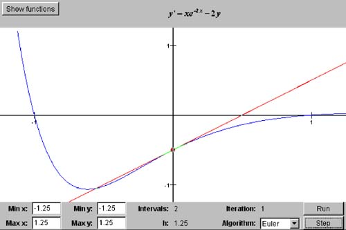
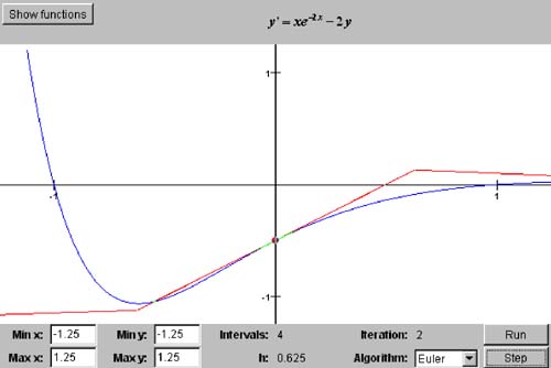
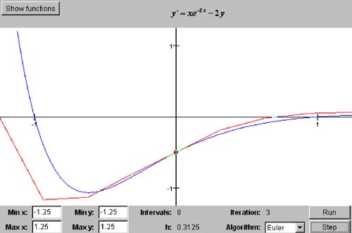
We can compute the next point ( x i + 1 , y i + 1 ) from the previous point ( x i , y i ) and the value of the slope y i ' = f ( x i , y i ) at the previous point. Review Figure 8-1. and, of course, x i + 1 = x i + h. Listing 8-0c shows the class DiffEqSolver in package numbercruncher. mathutils that will be the base class of the differential equation solver classes. Listing 8-0c The base class DiffEqSolver for the differential equation solver classes. package numbercruncher.mathutils; /** * The base class for differential equation solvers. */ public abstract class DiffEqSolver { /** the differential equation to solve */ protected DifferentialEquation equation; /** the initial condition data point */ protected DataPoint initialCondition; /** current x value */ protected float x; /** current y value */ protected float y; /** * Constructor. * @param equation the differential equation to solve */ public DiffEqSolver(DifferentialEquation equation) { this.equation = equation; this.initialCondition = equation.getInitialCondition(); reset(); } /** * Reset x and y to the initial condition data point. */ public void reset() { this.x = initialCondition.x; this.y = initialCondition.y; } /** * Return the next data point in the * approximation of the solution. * @param h the width of the interval */ public abstract DataPoint nextPoint(float h); } Instances of this abstract class store the differential equation and the initial condition, and they keep track of the current values of x and y . The abstract method nextPoint() will be implemented by the subclasses, where the method will compute and return the next data point based on the current values of x and y and value of the horizontal interval width h . Listing 8-1a Class EulersDiffEqSolver , the differential equation solver that implements Euler's algorithm. package numbercruncher.mathutils; /** * Differential equation solver that implements Euler's algorithm. */ public class EulersDiffEqSolver extends DiffEqSolver { /** * Constructor. * @param equation the differential equation to solve */ public EulersDiffEqSolver(DifferentialEquation equation) { super(equation); } /** * Return the next data point in the * approximation of the solution. * @param h the width of the interval */ public DataPoint nextPoint(float h) { y += h*equation.at(x, y); x += h; return new DataPoint(x, y); } } Listing 8-1a shows our first subclass of DiffEqSolver , class EulersDiffEqSolver in package numbercruncher.mathutils . As we can see, its nextPoint() method implements Euler's algorithm. The value of equation.at(x, y) is the slope at a point at one side of an interval, and the method returns the point at the other side of the interval. The noninteractive version of Program 8 §C1 works with different subclasses of DiffEqSolver , and which subclass it instantiates depends on the command-line argument processed by main() . In Listing 8-1b, we see its output with the command-line argument "eulers," which causes the program to instantiate a EulersDiffEqSolver object. Listing 8-1b The noninteractive version of Program 8 §C1 with the command-line argument "eulers" for Euler's algorithm. package numbercruncher.program8_1; import numbercruncher.mathutils.DifferentialEquation; import numbercruncher.mathutils.DataPoint; import numbercruncher.mathutils.DiffEqSolver; import numbercruncher.mathutils.EulersDiffEqSolver; import numbercruncher.mathutils.PredictorCorrectorDiffEqSolver; import numbercruncher.mathutils.RungeKuttaDiffEqSolver; import numbercruncher.mathutils.AlignRight; /** * PROGRAM 8-1: Solve Differential Equations * * Demonstrate algorithms for solving differential equations. */ public class SolveDiffEq { private static final int MAX_INTERVALS = Integer.MAX_VALUE/2; private static final int EULER = 0; private static final int PREDICTOR_CORRECTOR = 1; private static final int RUNGE_KUTTA = 2; private static final String ALGORITHMS[] = { "Euler's", "Predictor-Corrector", "Runge-Kutta" }; /** * Main program. * @param args the array of runtime arguments */ public static void main(String args[]) { String arg = args[0].toLowerCase(); int algorithm = arg.startsWith("eul") ? EULER : arg.startsWith("pre") ? PREDICTOR_CORRECTOR : RUNGE_KUTTA; System.out.println("ALGORITHM:"+ ALGORITHMS[algorithm]); solve(algorithm, "6x^2 - 20x + 11", 6); solve(algorithm, "2xe^2x + y", 1); solve(algorithm, "xe^-2x - 2y", 1); } private static void solve(int algorithm, String key, float x) { DifferentialEquation equation = DiffEqsToSolve.equation(key); DataPoint initialCondition = equation.getInitialCondition(); String solutionLabel = equation.getSolutionLabel(); float initX = initialCondition.x; float initY = initialCondition.y; float trueValue = equation.solutionAt(x); System.out.println(); System.out.println("Differential equation: f(x,y) ="+ key); System.out.println(" Initial condition: y(" + initX + ") ="+ initY); System.out.println(" Analytical solution: y ="+ solutionLabel); System.out.println(" True value: y(" + x + ") ="+ trueValue); System.out.println(); DiffEqSolver solver; switch (algorithm) { case EULER: { solver = new EulersDiffEqSolver(equation); break; } case PREDICTOR_CORRECTOR: { solver = new PredictorCorrectorDiffEqSolver(equation); break; } default: { solver = new RungeKuttaDiffEqSolver(equation); break; } } AlignRight ar = new AlignRight(); ar.print("n", 8); ar.print("h", 15); ar.print("y(" + x + ")", 15); ar.print("Error", 15); ar.underline(); int intervals = 2; float h = Math.abs(x - initX)/intervals; float error = Float.MAX_VALUE; float prevError; do { DataPoint nextPoint = null; for (int i = 0; i < intervals; ++i) { nextPoint = solver.nextPoint(h); } prevError = error; error = nextPoint.y - trueValue; ar.print(intervals, 8); ar.print(h, 15); ar.print(nextPoint.y, 15); ar.print(error, 15); ar.println(); intervals *= 2; h /= 2; solver.reset(); } while ((intervals < MAX_INTERVALS) && (Math.abs(prevError) > Math.abs(error))); } } Output: ALGORITHM: Euler's Differential equation: f(x,y) = 6x^2 - 20x + 11 Initial condition: y(0.0) = -5.0 Analytical solution: y = 2x^3 - 10x^2 + 11x - 5 True value: y(6.0) = 133.0 n h y(6.0) Error ----------------------------------------------------- 2 3.0 43.0 -90.0 4 1.5 74.5 -58.5 8 0.75 100.375 -32.625 16 0.375 115.84375 -17.15625 32 0.1875 124.21094 -8.7890625 64 0.09375 128.55273 -4.4472656 128 0.046875 130.76318 -2.2368164 256 0.0234375 131.87823 -1.1217651 512 0.01171875 132.43834 -0.56166077 1024 0.005859375 132.719 -0.28100586 2048 0.0029296875 132.85947 -0.14053345 4096 0.0014648438 132.92973 -0.07026672 8192 7.324219E-4 132.96489 -0.035110474 16384 3.6621094E-4 132.98236 -0.01763916 32768 1.8310547E-4 132.99138 -0.008621216 65536 9.1552734E-5 132.99562 -0.0043792725 131072 4.5776367E-5 132.99786 -0.0021362305 262144 2.2888184E-5 132.99792 -0.0020751953 524288 1.1444092E-5 133.0011 0.0010986328 1048576 5.722046E-6 133.00006 6.1035156E-5 2097152 2.861023E-6 133.03824 0.038238525 Differential equation: f(x,y) = 2xe^2x + y Initial condition: y(0.0) = 1.0 Analytical solution: y = 3e^x - 2e^2x + 2xe^2x True value: y(1.0) = 8.154845 n h y(1.0) Error ----------------------------------------------------- 2 0.5 3.6091409 -4.5457044 4 0.25 5.293519 -2.8613262 8 0.125 6.5289307 -1.6259146 16 0.0625 7.284655 -0.87019014 32 0.03125 7.7041717 -0.45067358 64 0.015625 7.9254375 -0.22940779 128 0.0078125 8.039102 -0.11574364 256 0.00390625 8.09671 -0.058135033 512 0.001953125 8.1257105 -0.02913475 1024 9.765625E-4 8.140253 -0.014592171 2048 4.8828125E-4 8.147548 -0.007297516 4096 2.4414062E-4 8.151206 -0.0036392212 8192 1.2207031E-4 8.153012 -0.001832962 16384 6.1035156E-5 8.15396 -8.8500977E-4 32768 3.0517578E-5 8.154387 -4.5776367E-4 65536 1.5258789E-5 8.154611 -2.3460388E-4 131072 7.6293945E-6 8.154683 -1.6212463E-4 262144 3.8146973E-6 8.154706 -1.3923645E-4 524288 1.9073486E-6 8.154436 -4.0912628E-4 Differential equation: f(x,y) = xe^-2x - 2y Initial condition: y(0.0) = -0.5 Analytical solution: y = (x^2e^-2x - e^-2x)/2 True value: y(1.0) = 0.0 n h y(1.0) Error ----------------------------------------------------- 2 0.5 0.09196986 0.09196986 4 0.25 0.043056414 0.043056414 8 0.125 0.02059899 0.02059899 16 0.0625 0.010078897 0.010078897 32 0.03125 0.00498614 0.00498614 64 0.015625 0.0024799863 0.0024799863 128 0.0078125 0.0012367641 0.0012367641 256 0.00390625 6.176049E-4 6.176049E-4 512 0.001953125 3.0862397E-4 3.0862397E-4 1024 9.765625E-4 1.5423674E-4 1.5423674E-4 2048 4.8828125E-4 7.712061E-5 7.712061E-5 4096 2.4414062E-4 3.8514103E-5 3.8514103E-5 8192 1.2207031E-4 1.9193667E-5 1.9193667E-5 16384 6.1035156E-5 9.6256945E-6 9.6256945E-6 32768 3.0517578E-5 4.7721633E-6 4.7721633E-6 65536 1.5258789E-5 2.3496477E-6 2.3496477E-6 131072 7.6293945E-6 9.0182266E-7 9.0182266E-7 262144 3.8146973E-6 -3.8416E-7 -3.8416E-7 524288 1.9073486E-6 4.7914605E-6 4.7914605E-6 Method solve() solves each initial value problem several times, each iteration with twice the number of intervals and half the horizontal interval width h . For each value of h , it repeatedly calls the nextPoint() method of the differential equation solver object. After each iteration, it tests the accuracy of the solution by evaluating the numerical solution function at a value of x some distance away from the initial x and then comparing the numerical solution with the true, analytical solution. The method has a unique stopping criterion. The error between the numerical solution and the true solution diminishes as the value of h decreases, until roundoff errors begin to dominate. The method stops the iteration when the error stops decreasing and begins to increase. The output of Listing 8-1b shows that Euler's algorithm converges slowly, and its accuracy can be low. Screen 8-1a shows screen shots of the interactive version [3] of Program 8 §C1, which can also work with different subclasses of DiffEqSolver . Here, we see the first three iterations of Euler's algorithm numerically solving the differential equation
Screen 8-1a. The first three iterations of Program 8 §C1 using Euler's algorithm to solve the initial value problem y ' = xe -2 x - 2 y and y (0) = -0.5. The analytical solution is the smooth curve, and the numerical solution consists of the line segments. The dot represents the initial condition. with the initial condition y (0) = -0.5. |

| |
| Top |
EAN: 2147483647
Pages: 141