5.2. Applications of DFs
| | ||
| | ||
| | ||
5.2. Applications of DFs
Due to their high information density, DFs have a huge number of applications. Among them are motion planning in robotics [Kimmel et al. 98, Latombe 91], collision detection, shape matching [Novotni and Klein 01], morphing [Cohen-Or et al. 98b], volumetric modeling [Frisken et al. 00, Bremer et al. 02, Youngblut et al. 02], navigation in virtual environments [Wan et al. 01], reconstruction [Klein et al. 99], offset surface construction [Payne and Toga 92], and dynamic levels of detail, to name but a few. In the following, we will highlight two easy applications of DFs.
5.2.1. Morphing
One interesting application of DFs is morphing, i.e., the problem of finding a smooth transition from a shape S ![]() to a shape T
to a shape T ![]() , i.e., we are looking for a shape transformation M ( t,
, i.e., we are looking for a shape transformation M ( t, ![]() ) , t ˆˆ [0 , 1], such that M (0 , S ) = S , M (1 , S ) = T .
) , t ˆˆ [0 , 1], such that M (0 , S ) = S , M (1 , S ) = T .
Sometimes, there is a bit of confusion about terms. Sometimes, morphing refers to any smooth transition. Other times, it refers only to those transitions that are bijective, continuous, and have a continuous inverse. In the latter case, the term morphing is equivalent to the notion of homeomorphism in the area of topology, and the term metamorphosis is used to refer to the broader definition. The difference between a homeomorphism and a metamorphosis is that the former does not allow you to cut or glue the shape during the transition (this would change the topology).
In the following, we will describe a simple method for metamorphosis of two shapes given as volumetric models; it was presented in [ ? ]. The nice thing about a volumetric representation is that it can naturally handle genus changes (i.e., the number of holes in S and T is different).
In the simplest form, we can just interpolate linearly between the two DFs of S and T , yielding a new DF
| (5.3) | |
In order to obtain a polygonal representation, we can compute the isosurface for the value 0.
This works quite well, if S and T are aligned with each other (in an intuitive sense). However, when morphing two sticks that are perpendicular to each other, there will be in-between models that almost vanish .
Therefore, in addition to the DF interpolation, we usually want to split the morphing into two steps (for each t ): first, S is warped by some function W ( t, x ) into S , then D S and D T are interpolated, i.e., M ( t , S ) = tD W(t , S) + (1 ˆ t ) D T .
The idea of the warp is that it encodes the expertise of the user who usually wants a number of prominent feature points from S to transition onto other feature points on T . For instance, she wants the corresponding tips of nose, fingers, and feet of two different characters to transition into each other.
Therefore, we must specify a small number of correspondences ( p ,i , p 1 ,i ), where p ,i ˆˆ S , and p 1 ,i ˆˆ T (see Figure 5.7). Then we determine a warp function W ( t, x ) such that W (1 , p ,i ) = p 1 ,i .
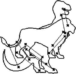
Figure 5.7: By specifying correspondences, the user can identify feature points that should transition into each other during the morph [?]. (Courtesy of Daniel Cohen-Or.)
Since the warp function should distort S as little as possible (just align them), we can assemble it from a rotation, then a translation, and finally an elastic part that is not a linear transformation:
| (5.4) | |
where E is the elastic transformation, R ( a , ) is a rotation about axis a and angle , and c is the translation.
The rotation and translation of the warp function can be determined by least-squares fitting, while the elastic transformation can be formulated as a scattered data interpolation problem. One method that has proven quite robust is the approach using radial basis functions. The interested reader will find the details in [ ? ].
5.2.2. Modeling
A frequently used modeling paradigm in CAD is volumetric modeling , which means that objects are, conceptually, defined by specifying for each point whether or not it is a member of the object. The advantage is that it is fairly simple to define Boolean operations on such a representation, such as union, subtraction, and intersection. Examples of volumetric modeling is constructive solid geometry (CSG) and voxel-based modeling . The advantage of using DFs for volumetric modeling is that they are much easier to implement than CSG, but provide much better quality than simple voxel-based approaches.
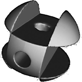
Figure 5.9: Example of a 3D difference operation [Bremer et al. 02]. (Courtesy of Prof. Bremer et al.)
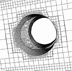
Figure 5.10: Close-up view showing the adaptivity [Bremer et al. 02]. (Courtesy of Prof. Bremer et al.)
Computing the Boolean operation on two DFs basically amounts to evaluating the appropriate operator on the two fields. The following table gives these operators for a field D O (for the object) and a field D T (for the tool):
| Boolean operation | Operator on DF |
|---|---|
| Union | D O ˆ T = min( D O , D T ) |
| Intersection | D O ˆ T = max( D O , D T ) |
| Difference | D O ˆ T = max( D O , ˆ D T ) |
Figure 5.8 shows an example of the difference operation.
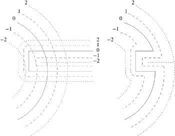
Figure 5.8: Example of difference of two DFs. On the left, the two DFs for tool and object are shown superimposed; on the right, the result is shown.
If ADFs are used for representation of the DFs, then a recursive procedure has to be applied to the objects ADF to compute the resulting ADF. It is similar to the generation of ADFs (see Section 5.1) except that here the subdivision is governed by the compliance of new object ADF with the tool ADF: a cell is further subdivided if it contains cells from the tool ADF that are smaller and if the trilinear interpolation inside the cell does not approximate well enough the ADF of the tool.
EAN: N/A
Pages: 69