5.1. Computation and Representation of DFs

For special surfaces S , we may be able to compute D _S analytically. In general, however, we have to discretize D _S spatially, i.e., store the information in a 3D voxel grid, octree, or other space partitioning data structure. Voxel grids and octrees are the most commonly used data structures for storing DFs, and we will describe algorithms for them in the following sections. More sophisticated representations try to store more information at each voxel in order to be able to extract distances quickly from the field [Huang et al. 01].

Since each cell in a discrete DF stores one signed distance to the surface for only one representative, the distance of other points must be interpolated from these values. One simple method is to store exact distances for the nodes (i.e., the corners of the voxels), and generate all other distances in the interior of voxels by trilinear interpolation. Other interpolation methods could be used as well.

The simplest discrete representation of a DF is the 3D voxel grid. However, for most applications, this is too costly, not only in memory utilization but also in computational efforts. So, usually DFs are represented using octrees (see Figure 5.4), because they are simple to construct, offer fairly good adaptivity, and allow for easy algorithms [Frisken et al. 00, ? ]. This representation is called an adaptively sampled distance field (ADF). Actually, the kind of hierarchical space partitioning is a design parameter of the algorithm; for instance, BSPs (see Chapter 3) probably offer much more efficient storage at the price of more complex interpolation.

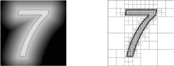
Figure 5.4: Representing distance fields (left: 2D field of the number 7, 262,144 distance samples) by octrees (right: quadtree cells are subdivided to their highest resolution along the boundary of the 2D shape, yielding 6681 cells ) has both memory and computational advantages. (Courtey of Sarah Frisken, Tufts University, and Ronald Perry, Mitsubishi Electric Research Laboratories.)

Constructing ADFs works much like constructing regular octrees for surfaces, except that here, we subdivide a cell if the DF is not well approximated by the interpolation function defined so far by the cell corners.

The following two algorithms for computing a DF produce only flat representations (i.e., grids), but they can be turned into an ADF by coalescing cells in a bottom-up manner if the resulting cell still describes the DF well enough. ^[2]

5.1.1. Propagation Method

The propagation method bears some resemblance to region growing and flood filling algorithms, and is also called the chamfer method . It can produce only approximations of the exact DF.

The idea is to start with a binary DF, where all voxels intersecting the surface are assigned a distance of 0, and all others are assigned a distance of ˆ . Then we somehow propagate these known values to voxels in the neighborhood, taking advantage of the fact that we already know the distances between neighboring voxels. ^[3] Note that these distances depend on only the local neighborhood constellation, no matter where the propagation front currently is.

More formally speaking, since we want to compute the DF for only a discrete set of points in space, we can reformulate Equation (5.1) as follows :

(5.2)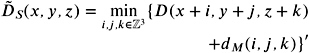

where d _M is the distance of a node ( i, j, k ) from the center node (0 , , 0). Actually, this is already a slight approximation of the exact DF.

We can now further approximate this by not considering the infinite neighborhood ( i, j, k ) ˆˆ , but only a local one . Since a practical computation of would compute each node in some kind of scan order, we choose such that it contains only nodes that have already been computed by the respective scan. Thus, d _M can be precomputed and stored conveniently in a 3D matrix (see Figure 5.5).

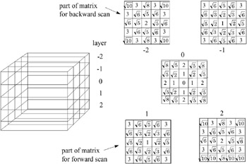
Figure 5.5: By convoluting a distance matrix with an initially binary distance field (0 or ˆ ), one gets an approximate distance field. Here, a 5 — 5 — 5 example of such a matrix is shown.

This process looks very similar to conventional convolution, except that here we perform a minimum operation over a number of sums; the conventional convolution performs a sum over a number of products.

Obviously, a single scan will not assign meaningful distance values to all nodes, no matter in what order the scan performs. Therefore, we need at least two scans : for instance, first, a 3D scanline order from top to bottom (forward), and second, backward from bottom to top. In each pass, only one half of the 3D matrix d _M needs to be considered (see Figure 5.5). Of course, there could still be nodes with distance ˆ in the respective part of the chamfer matrix.

The time complexity of this method is in O ( m ), m = number of voxels. However, the result is only an approximation of the DF; in fact, the accuracy of the distance values can be pretty low. ^[4]

In order to further improve accuracy, one can make a few more passes , not only from top to bottom and back, but also from left to right, etc. Another option is to increase the size of d _M .

Analogously, an approximate vector DF can be computed [Jones and Satherly 01]. In that case, the matrix d _M contains vectors instead of scalars. To improve the accuracy, we can proceed in two steps: first, for each voxel in the neighborhood of the surface (usually just the 3 ³ neighborhood), we compute vectors to the exact closest point on the surface; then this shell is propagated by several passes with the vector-valued matrix d _M . The time for computing the exact distance shell can be optimized by utilizing an octree or BVH for closest point computation, and initializing each search with the distance (and vector) to the closest point of a nieghbor voxel.

5.1.2. Projection of Distance Functions

The propagation method described in the previous section can be applied to all kinds of surfaces S . However, it can produce only very gross approximations. Here, we describe a method that can produce much better approximations. However, it can be applied only to polygonal surfaces S .

The key technique applied in this approach is to embed the problem into more dimensions than are inherent in the input/output itself. This is a very general technique that often helps to get a better and simpler view on a complex problem.

The method described here was presented in [Hoff III et al. 99] and [Haeberli 90], and, from a different point of view, in [Sethian 96].

Let us consider the DF of a single point in 2D. If we consider this a surface in 3D, then we get a cone with the apex in that point. In other words, the DF of a point in a plane is just the orthogonal projection of suitable cone onto the plane z = 0.

Now, if there are n point sites in the plane, we get n cones, so each point in the plane will be hit by n distance values from the projection (see Figure 5.6(left)). Obviously, only the smallest one wins and gets stored with that pointand this is exactly what the Z-buffer of graphics hardware was designed for.

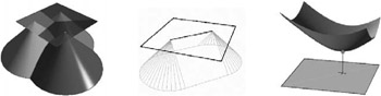
Figure 5.6: (left) The distance function of a point site in the plane is a cone. (middle) More complex sites have a bit more complex distance functions. (right) The distance function of sites in 3D is different for the different slices of the volume [Hoff III et al. 99]. (See Color Plate IX.) (Courtesy of K. Hoff, T. Culver, J. Keyser, M. Lin, and D. Manocha, Copyright ACM.)

These cones are called the distance function for a point. The distance function for other features (line segments, polygons, and curves) is a little more complicated (see Figure 5.6(middle)).

So, computing a discrete DF for a set of sites in the plane can be done by rendering all the associated distance functions (represented as polygonal meshes) and reading out the Z-buffer (and possibly the frame buffer if we also want the site IDs, i.e., discretized Voronoi regions ). If we want to compute a 3D DF, then we proceed slice by slice. One noteworthy catch, though, is that the distance functions of the sites change from slice to slice. For instance, the distance function for a point that lies not in the current slice is a hyperboloid, with the point site being coincident with the vertex of the hyperboloid (see Figure 5.6(right)).

^[2] Usually, it is faster to compute an ADF top-down, though.

^[3] This idea has been proposed as early as 1984 [Borgefors 84], and maybe even earlier.

^[4] Furthermore, the distance values are not even an upper bound on the real distance.