Organizing Data into Levels

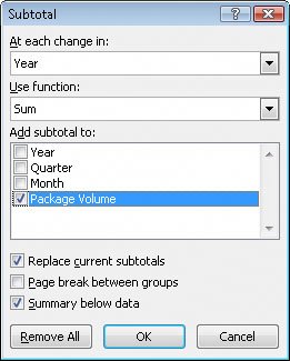
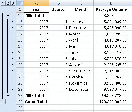
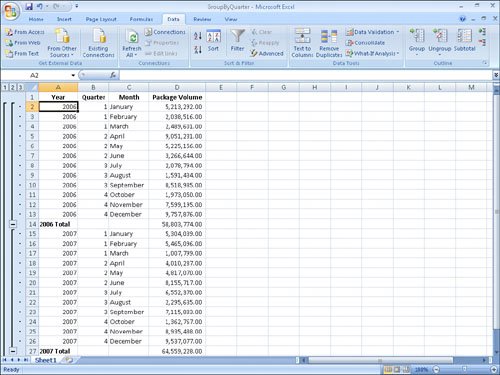
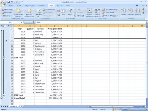
After you have sorted the rows in an Excel 2007 worksheet or entered the data so that it doesn't need to be sorted, you can have Excel 2007 calculate subtotals or totals for a portion of the data. In a worksheet with sales data for three different product categories, for example, you can sort the products by category, select all the cells that contain data, and then open the Subtotal dialog box. To open the Subtotal dialog box, display the Data tab and then, in the Outline group, click Subtotal.

In the Subtotal dialog box, you can choose the column on which to base your subtotals (such as every change of value in the Week column), the summary calculation you want to perform, and the column or columns with values to be summarized. In the worksheet in the preceding graphic, for example, you could also calculate subtotals for the number of units sold in each category. After you define your subtotals, they appear in your worksheet.

As the graphic shows, when you add subtotals to a worksheet, Excel 2007 also defines groups based on the rows used to calculate a subtotal. The groupings form an outline of your worksheet based on the criteria you used to create the subtotals. In the preceding example, all the rows representing months in the year 2006 are in one group, rows representing months in 2007 are in another, and so on. The outline section at the left of your worksheet holds controls you can use to hide or display groups of rows in your worksheet.

There are three types of controls in the outline section: Hide Detail buttons, Show Detail buttons, and level buttons.

The Hide Detail button beside a group can be clicked to hide the rows in that group. In the previous graphic, clicking the Hide Detail button next to row 27 would hide rows 15 through 26 but leave the row holding the subtotal for that group, row 27, visible.

When you hide a group of rows, the button next to the group changes to a Show Detail button. Clicking a group's Show Detail button restores the rows in the group to the worksheet.

The level buttons comprise the other set of buttons in the outline section of a worksheet with subtotals. Each button represents a level of organization in a worksheet; clicking a level button hides all levels of detail below that of the button you clicked. The following table identifies the three levels of organization shown in the preceding graphic.

Level	Description
1	Grand total
2	Subtotals for each group
3	Individual rows in the worksheet

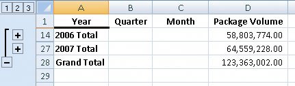
Clicking the Level 2 button in the worksheet shown in the preceding illustration would hide the rows with data on each month's revenue but would leave the row that contains the grand total (Level 1) and all rows that contain the subtotal for each year (Level 2) visible in the worksheet.

If you like, you can add levels of detail to the outline that Excel 2007 creates. For instance, you might want to be able to hide revenues from January and February, which you know are traditionally strong months. To create a new outline group within an existing group, select the rows you want to group; on the Data tab, in the Outline group, point to Group and Outline, and then click Group.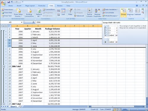

You can remove a group by selecting the rows in the group and clicking Ungroup from the Data tab Outline group.

Tip

If you want to remove all subtotals from a worksheet, open the Subtotal dialog box and click the Remove All button.

In this exercise, you will add subtotals to a worksheet and then use the outline that appears to show and hide different groups of data in your worksheet.

USE the GroupByQuarter workbook in the practice file folder for this topic. This practice file is located in the My Documents\Microsoft Press\Excel SBS\Sorting folder.

OPEN the GroupByQuarter workbook.

1.	Click any cell in the data list.
2.	On the Data tab, in the Outline group, click Subtotal. The Subtotal dialog box appears with the default options to add a subtotal at every change in the Year column, to return the sum of the values in the subtotaled rows, and to add a row with the subtotal of values in the Package Volume column below the final selected row.
3.	Click OK. The Subtotal dialog box disappears. New rows appear with subtotals for package volume during each year represented in the worksheet. The new rows are numbered 14 and 27. A row with the grand total of all rows also appears; that row is row 28. A new section with outline bars and group-level indicators appears to the left of column A.
4.	Click the row head button of row 5 and drag to the row head button of row 7. Rows 5 through 7 are highlighted.
5.	On the Data tab, in the Outline group, click Group. Rows 5 through 7 are made into a new group. An outline bar appears on a new level in the outline section, and a corresponding Level 4 button appears at the top of the outline section.
6.	In the outline section, click the Hide Detail button next to row 8. Rows 5 through 7 are hidden, and the Hide Detail button you clicked changes to a Show Detail button.
7.	In the outline section, click the Show Detail button next to row 8. Rows 5 through 7 reappear.
8.	In the outline section, click the Level 1 button. All rows except row 1 with the column headings and row 28 with the grand total are hidden.
9.	In the outline section, click the Level 2 button. The rows with the subtotal for each week appear.
10.	In the outline section, click the Level 3 button. All rows except rows 5 through 7 appear.
11.	In the outline section, click the Level 4 button. Rows 5 through 7 reappear.

CLOSE the GroupByQuarter workbook.