Sorting Data Lists

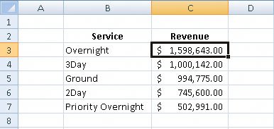
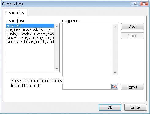
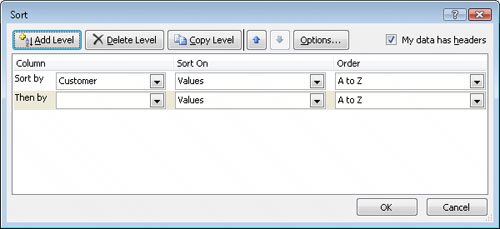
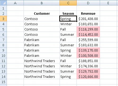
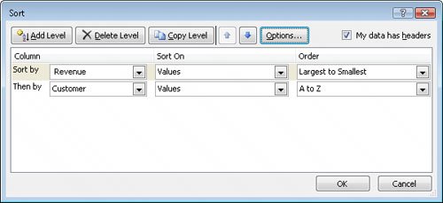
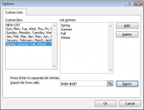
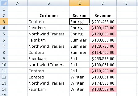
Although Excel 2007 makes it easy to enter your business data and to manage it after you've saved it in a worksheet, your data will rarely answer every question you want to ask it. For example, you might want to discover which of your services generates the most profits, which service costs the most for you to provide, and so on. You can find out that information by sorting your data.

When you sort data in a worksheet, you rearrange the worksheet rows based on the contents of cells in a particular column. Sorting a worksheet to find your highest-revenue services might show the results displayed in the following graphic.

You can sort a group of rows in a worksheet in a number of ways, but the first step is to identify the column that will provide the values by which the rows should be sorted. In the preceding graphic, you could find the highest revenue totals by selecting the cells in the Revenue column and displaying the Home tab of the user interface. Then, in the Editing group, click Sort & Filter and click Sort Descending. Clicking Sort Descending makes Excel 2007 put the row with the highest value in the Revenue column at the top of the worksheet and continue down to the lowest value.

If you want to sort the rows in the opposite order, from the lowest revenue to the highest, select the cells in the Revenue column and then, from the Editing group Sort & Filter button list, click Sort Ascending.

The Sort Ascending and Sort Descending buttons enable you to sort rows in a worksheet quickly, but you can use them only to sort the worksheet based on the contents of one column, even though you might want to sort by two columns. For example, you might want to order the worksheet rows by service category and then by total so that you can see the customers that use each service category most frequently. You can sort rows in a worksheet by the contents of more than one column through the Sort dialog box, in which you can pick any number of columns to use as sort criteria and choose whether to sort the rows in ascending or descending order.

To display the Sort dialog box, display the Home tab and then, in the Editing group, click Sort & Filter and then click Custom Sort.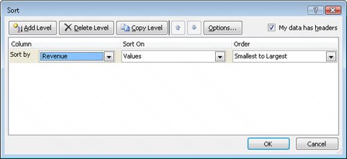

If your data list has a header row, select the My data has headers check box so the column headers will appear when you click the Column down arrow next to the Sort by field. After you set the column by which you want to sort, clicking the Sort On field down arrow enables you to select whether you want to sort by a cell's value (the default), a cell's fill color, a cell's font color, or an icon displayed in the cell.

See Also

For more information on creating conditional formats that change a cell's formatting or display icon sets to reflect the cell's value, refer to "Changing the Appearance of Data Based on Its Value" in Chapter 5.

Finally, you can click the Order field down arrow to select how you want Excel 2007 to sort the column values. The exact list changes to reflect the data in your column. If your column contains numerical values, you'll see the options Largest to Smallest, Smallest to Largest, and Custom List. If your column contains text values, the options will be A to Z (ascending order), Z to A (descending order), and Custom List. And if your column contains dates, you'll see Newest to Oldest, Oldest to Newest, and Custom List.

Adding, moving, copying, and deleting sorting levels are a matter of clicking the appropriate button in the Sort dialog box. To manage a data range's sorting levels, click the Add Level button.

Note

In previous versions of Excel, you could create a maximum of three sorting levels. You may create up to 64 sorting levels in Excel 2007.

The Sort dialog box appears with fields to create one sorting level. To create a new level, click Add Level. To delete a level, click the level in the list and then click Delete Level. Clicking Copy Level enables you to put all the settings from one rule into another, saving you some work if you need to change only one item. The Move Up and Move Down buttons, which display an upward-pointing arrow and a downward-pointing arrow, respectively, enable you to change a sorting level's position in the order. Finally, clicking the Options button displays the Sort Options dialog box, which you can use to make a sorting level case sensitive.

The default setting for Excel 2007 is to sort numbers according to their values and to sort words in alphabetical order, but that pattern doesn't work for some sets of values. One example in which sorting a list of values in alphabetical order would yield incorrect results is with the months of the year. In an "alphabetical" calendar, April is the first month, and September is the last! Fortunately, Excel 2007 recognizes a number of special lists, such as days of the week and months of the year. You can have Excel 2007 sort the contents of a worksheet based on values in a known list; if needed, you can create your own list of values. For example, the default lists of weekdays in Excel 2007 start with Sunday. If you keep your business records based on a MondaySunday week, you can create a new list with Monday as the first day and Sunday as the last.

To create a new list, type the list of values you want to use as your list into a contiguous cell range, select the cells, click the Microsoft Office Button, and then click Excel Options. On the Popular page of the dialog box, click the Edit Custom Lists button to display the Custom Lists dialog box.

The selected cell range's reference appears in the Import list from cells field. To record your list, click the Import button.

Note

Another benefit of creating a custom list is that dragging the fill handle of a list cell that contains a value causes Excel 2007 to extend the series for you. For example, if you create the list Spring, Summer, Fall, Winter, type Summer in a cell, and then drag the cell's fill handle; Excel 2007 extends the series as Fall, Winter, Spring, Summer, Fall, and so on.

To use a custom list as a sorting criterion, display the Sort dialog box, click the rule's Order field down arrow, click Custom List, and select your list from the dialog box that appears.

Important

In previous versions of Excel, your custom list had to be the primary sorting criterion. In Excel 2007, you can use your custom list as any criterion.

In this exercise, you will sort a data list, sort a list by multiple criteria, change the order in which sorting criteria are applied, sort data by using a custom list, and sort data by color.

USE the ShippingSummary workbook in the practice file folder for this topic. This practice file is located in the My Documents\Microsoft Press\Excel SBS\Sorting folder.

BE SURE TO start Excel 2007 before beginning this exercise.

OPEN the ShippingSummary workbook.

1.	Click cell C3.
2.	On the Home tab, in the Editing group, click Sort & Filter and then click Sort A to Z. Excel 2007 sorts the data by season.
3.	On the Home tab, in the Editing group, click Sort & Filter and then click Custom Sort. The Sort dialog box appears.
4.	Select the My data has headers check box.
5.	Click the Column field down arrow and then click Customer. If necessary, click the Sort On field down arrow and click Values; then click the Order field down arrow and click A to Z.
6.	Click Add Level. A new Then by sorting level appears.
7.	Click the new Column field down arrow and then click Revenue.
8.	Click the new Order field down arrow and then click Largest to Smallest.
9.	Click OK. Excel 2007 closes the Sort dialog box and sorts the data list.
10.	On the Home tab, in the Editing group, click Sort & Filter and then click Custom Sort. The Sort dialog box appears.
11.	Click Then by. Excel 2007 highlights the second sorting rule.
12.	Click the Move Up button. Excel 2007 moves the second sorting rule above the first.
13.	Click OK. Excel 2007 closes the Sort dialog box and sorts the data list.
14.	Select cells G4:G7, click the Microsoft Office Button and then click Excel Options. The Excel Options dialog box appears.
15.	On the Popular tab, click Edit Custom Lists. The Custom Lists dialog box appears.
16.	Verify that the cell range $G$4:$G$7 appears in the Import list from cells field and then click Import. The new list appears in the Custom lists pane.
17.	Click OK twice to close the Custom Lists dialog box and the Excel Options dialog box.
18.	Click cell C3.
19.	On the Home tab, in the Editing group, click Sort & Filter and then click Custom Sort. The Sort dialog box appears.
20.	Click the rule in the Sort by row and then click Delete Level. The sorting rule disappears.
21.	In the Sort by row, click the Column field down arrow and then click Season.
22.	In the same row, click the Order field down arrow and then click Custom List. The Custom Lists dialog box appears.
23.	In the Custom lists pane, click the sequence Spring, Summer, Fall, Winter.
24.	Click OK twice to close the Custom Lists dialog box and the Sort dialog box. Excel 2007 sorts the data list.
25.	Click cell C3 and then, on the Home tab, in the Editing group, click Sort & Filter and then click Custom Sort. The Sort dialog box appears.
26.	In the Sort by row, click the Sort by field down arrow and then click Revenue.
27.	Click the Sort on field down arrow and then click Cell Color.
28.	Click the final field in the Sort by row and then click On Bottom to have Excel 2007 put the Revenue cells that have no cell color on the bottom.
29.	Click OK. Excel 2007 sorts the data list.

CLOSE the ShippingSummary workbook.