Section 09. Chi-Square

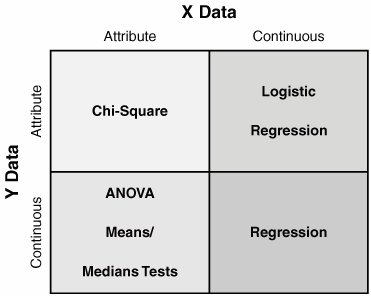
09. Chi-Square

Overview

Chi-square is one of the statistical tools in the Multi-Vari approach and is both the simplest and least powerful. Chi-square helps determine the statistical significance of a relationship between an Attribute X and an Attribute Y in Y = f(X₁,X₂,..., X_n).

The approach used is to assume the variables are independent and set up the hypotheses as follows:

H_o: Data are Independent (Not Related)
H_a: Data are Dependent (Related)

The output of the test is a "p-value" that indicates the likelihood of seeing a relationship this strong in a sample purely by random chance; that is, there is no relationship at the population level, it just happened by fluke in selecting the sample from the population. As in most statistical tests, if the p-value is less than 0.05, then the null hypothesis H_o should be rejected. In English, if the p is less than 0.05, then the likelihood of seeing a relationship this strong is less than 5%, and, therefore, there is a good chance that it is real; if p is greater than 0.05 then the conclusion should be that there is no relationship.

As with any statistical test, Chi-square comes with its set of "could be" and "might be" statements.

For example if the Personnel Department wants to see if there is a link between age and whether an applicant is hired, then both Age (old and young) and Got Hired (did or didn't) are attribute type data. A Chi-Square test would be applicable to answer the questions:

Are age and hiring decisions dependent or independent?
Does an association exist between age and hiring practice?
Is one age-group more likely than the other to get hired, or is the chance of getting hired independent of age?

The hypotheses would be

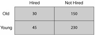
H_o: Age and Hiring Decisions are independent
H_a: Age and Hiring Decisions are dependent

As with all statistical tests, a sample of reality is required, similar to that shown in Table 7.09.1 where about 455 data points were taken and the data distributed amongst the four possible outcomes.

The data can then be analyzed in a statistical package, such as JMP or Minitab. The software calculates the expected values in each box, and compares the observed with the expected frequencies to produce a signal-to-noise type ratio (how far the observed is from the expected) using

Where O is the observed frequency and E is the expected frequency in a box.

Table 7.09.1. Sample of Reality for the Relationship between Age and Hiring

The software then looks up the χ² (the sum of all the discrepancies) value in a statistical table to discover the likelihood of seeing a difference that big.^[14] As a Belt using the tool practically, all that is important, after the data has been captured using robust data collection methods, is the output of the tool, which should be similar to that shown in Figure 7.09.1.

^[14] For more detail on exactly how this is calculated see Statistics for Management and Economics by Keller and Warrack.

Figure 7.09.1. Results of the Chi-Square test for the relationship between Age and Hiring Practice (output from Minitab v14).
Chi-Square Test: Hired, Not Hired
Expected counts are printed below observed counts Chi-Square contributions are printed below expected counts
	Hired	Not Hired	Total
1	30	150	180
	29.67	150.33
	0.004	0.001
2	45	230	275
	45.33	229.67
	0.002	0.000
Total	75	380	455
Chi-Sq = 0.007, DF = 1, P-Value = 0.932

The first place to look is the p-value, which in this case p = 0.932. In this instance, the p-value is not low (not below 0.05); thus, the conclusion should be that the relationship between Age and Hiring Practice is not significant for the sample of data taken.

Chi-Square can be applied in virtually any transactional processes where attribute data usually abounds. For example:

HR Number of sick days by employee or department
Accounting Number of incorrect expense reports by employee or department
Sales Number of lost sales by account or region or country
Logistics Number of deliveries late by distribution center or country
Call Center Number of missed Customer calls by associate or shift
Installation Number of repeat service calls by field technician
Purchasing Number of days delivery-time for orders by supplier
Inventory Number of parts by distribution center

Roadmap

The roadmap to setting up and applying a Chi-Square test is as follows:

Step 1.	Understand the question at hand. There should be a clear relationship in question; does X affect Y? The relationship needs to involve data for both X and Y that is attribute or discrete valued. There should be a business reason for asking the question in the first place, that is the question "Why do we care?" needs to have been answered.
Step 2.	Set up the hypotheses in the form: H_o: Data are Independent (Not Related) H_a: Data are Dependent (Related)
Step 3.	Determine a data collection method and a sample size. The sample size is based on the expected values in each box in the data collection table. To have a reasonable confidence in the result of the test, there needs to be an expected value in each box greater than 5. Thus, to calculate sample size, identify the lowest potential proportion likely in any of the boxes. Divide 5 by this proportion to give an approximate bare minimum number of data points to collect. For example, if the expected proportion in one box is 2.5% (0.025), then dividing 5 by 0.025 gives 200 data points. This is a little hit and miss, but gives a ballpark approximation. Typically the approach is to double this number to be on the safe side. The Chi-Squared test is data hungry, with sample sizes often above 500. A simple Tally Sheet is enough to capture most test data, placing check marks in the appropriate box as a data point is collected.
Step 4.	Collect the sample of reality. Ideally the data is available historically, or available quickly in large quantities or otherwise the project might need to idle while data is collected.
Step 5.	The data is entered in the form of a table into a statistical package and analyzed.

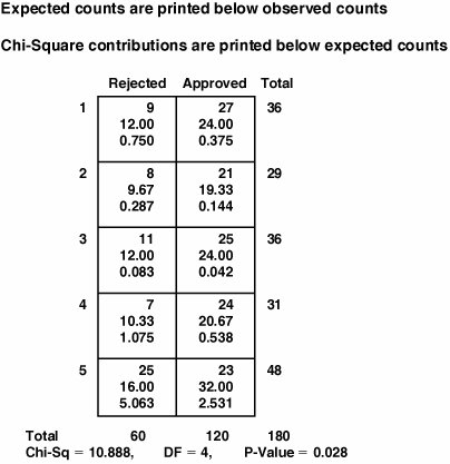
Interpreting the Output

The first place to look during analysis is to the p-value. If the p-value is higher than 0.05 then the conclusion is that the X and Y are not dependent based on the sample of reality taken (similar to the Age versus Hiring Practice example in "Overview" in this section).

However, if the p-value is low (less than 0.05) then there is reason to believe that the X and Y are dependent in some way and the distribution of data points within the table isn't as expected if everything was based on random chance.

To demonstrate this, consider the data in Table 7.09.2, which represents loan approval or rejection decisions on different days of the week. The bank in question clearly would like loan decisions to be independent of the day the loan was processed.

Table 7.09.2. Loan Decision Data by Day of Week
	Rejected	Approved
Monday	9	27
Tuesday	8	21
Wednesday	11	25
Thursday	7	24
Friday	25	23

The results of the Chi-Square Test analysis are shown in Figure 7.09.2.

Figure 7.09.2. Chi-Square Test analysis results for loan data (output from Minitab v14).

Looking immediately to the p-value of 0.028 (less than 0.05), it is clear that the likelihood of seeing a distribution of data in the boxes like this purely by random chance, given that there was no relationship, is slim. Thus, the conclusion is that the null hypothesis should be rejected and the alternate "Data are dependent" should be accepted instead. In English, we conclude there is something fishy going on, because the chances of getting a loan varies by day of the week.

To understand how this is manifested, the next step is to look to the contingency table in the analysis output as shown in Figure 7.09.2. To read this table, the numbers 1 to 5 down the left side represent the days Monday to Friday. The first number in each box is the observed data; that is how the decisions were actually made. The second number in each box is what would be expected if the decision were independent of the day. The final number is the Chi-Square statistic for the difference of the Observed versus the Expected values; the larger the number, the bigger the signal that is present.

Looking at the table it is clear that Friday has the larger deviation from expected, and this is contributing most of the Chi-Square total (5.063 + 2.531 out of 10.888). Looking at the observed versus expected values in the Friday row shows for Rejection an expected of 16 and an observed of 25; it seems on Friday a significant number of people get rejected more than we would expect.

The next steps would be to

See if, by omitting Friday's data and analyzing just the Monday to Thursday data, the other days of the week show a problem (in fact they don't).
Seek to understand the practical implications of Friday being different; that is, what causes the Friday phenomenon (perhaps the staff doesn't want to get bogged down in paperwork on a Friday afternoon and wants to get out early). The Belt can't jump to any conclusions here and should play detective to determine the real reasons.