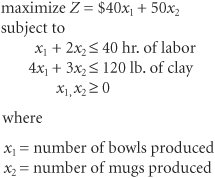
Goal Programming | Introduction to Management Science (10th Edition)

[Page 390 ( continued )]

As we mentioned, a goal programming model is very similar to a linear programming model, with an objective function, decision variables, and constraints. Like linear programming, goal programming models with two decision variables can be solved graphically and by using QM for Windows and Excel. We begin our presentation of goal programming as we did linear programming, demonstrating through an example of how to formulate a model. This will illustrate the main differences between goal and linear programming.

Model Formulation

We will use the Beaver Creek Pottery Company example again to illustrate the way a goal programming model is formulated and the differences between a linear programming model and a goal programming model. Recall that this model was originally formulated in Chapter 2 as follows :

The objective function, Z , represents the total profit to be made from bowls and mugs, given that $40 is the profit per bowl and $50 is the profit per mug. The first constraint is for available labor. It shows that a bowl requires 1 hour of labor, a mug requires 2 hours, and 40 hours of labor are available daily. The second constraint is for clay, and it shows that each bowl requires 4 pounds of clay, each mug requires 3 pounds , and the daily limit of clay is 120 pounds .

[Page 391]

This is a standard linear programming model; as such, it has a single objective function for profit. However, let us suppose that instead of having one objective, the pottery company has several objectives, listed here in order of importance :

To avoid layoffs, the company does not want to use fewer than 40 hours of labor per day.
The company would like to achieve a satisfactory profit level of $1,600 per day.
Because the clay must be stored in a special place so that it does not dry out, the company prefers not to keep more than 120 pounds on hand each day.
Because high overhead costs result when the plant is kept open past normal hours, the company would like to minimize the amount of overtime.

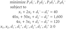
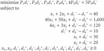
These different objectives are referred to as goals in the context of the goal programming technique. The company would, naturally, like to come as close as possible to achieving each of these goals. Because the regular form of the linear programming model presented in previous chapters considers only one objective, we must develop an alternative form of the model to reflect these multiple goals. Our first step in formulating a goal programming model is to transform the linear programming model constraints into goals.

The different objectives in a goal programming problem are referred to as goals.

Labor Goal

The first goal of the pottery company is to avoid underutilization of laborthat is, using fewer than 40 hours of labor each day. To represent the possibility of underutilizing labor, the linear programming constraint for labor, x ₁ + 2 x ₂ 40 hours of labor, is reformulated as

This reformulated equation is referred to as a goal constraint . The two new variables, d ₁ and d ₁ ⁺ , are called deviational variables . They represent the number of labor hours less than 40 ( d ₁ ) and the number of labor hours exceeding 40 ( d ₁ ⁺ ). More specifically , d ₁ represents labor underutilization, and d ₁ ⁺ represents overtime . For example, if x ₁ = 5 bowls and x ₂ = 10 mugs, then a total of 25 hours of labor have been expended. Substituting these values into our goal constraint gives

All goal constraints are equalities that include deviational variables, d and d ⁺ .

Because only 25 hours were used in production, labor was underutilized by 15 hours (40 - 25 = 15). Thus, if we let d ₁ = 15 hours and d ₁ ⁺ = 0 (because there is obviously no overtime), we have

A positive deviational variable (d ⁺ ) is the amount by which a goal level is exceeded .

A negative deviational variable (d) is the amount by which a goal level is underachieved .

Now consider the case where x ₁ = 10 bowls and x ₂ = 20 mugs. This means that a total of 50 hours have been used for production, or 10 hours above the goal level of 40 hours. This extra 10 hours is overtime. Thus, d ₁ = 0 (because there is no underutilization) and d ₁ ⁺ = 10 hours.

In each of these two brief examples, at least one of the deviational variables equaled zero. In the first example, d ₁ ⁺ = 0, and in the second example, d ₁ = 0. This is because it is impossible to use fewer than 40 hours of labor and more than 40 hours of labor at the same time . Of course, both deviational variables, d ₁ and d ₁ ⁺ , could have equaled zero if exactly 40 hours were used in production. These examples illustrate one of the fundamental characteristics of goal programming: At least one or both of the deviational variables in a goal constraint must equal zero.

[Page 392]

At least one or both deviational variables in a goal constraint must equal zero .

The next step in formulating our goal programming model is to represent the goal of not using fewer than 40 hours of labor. We do this by creating a new form of objective function:

minimize P ₁ d ₁

The objective function in all goal programming models is to minimize deviation from the goal constraint levels. In this objective function, the goal is to minimize d ₁ , the underutilization of labor. If d ₁ equaled zero, then we would not be using fewer than 40 hours of labor. Thus, it is our objective to make d ₁ equal zero or the minimum amount possible. The symbol P ₁ in the objective function designates the minimization of d ₁ as the first-priority goal. This means that when this model is solved, the first step will be to minimize the value of d ₁ before any other goal is addressed.

The objective function in a goal programming model seeks to minimize the deviation from goals in order of the goal priorities .

The fourth-priority goal in this problem is also associated with the labor constraint. The fourth goal, P ₄ , reflects a desire to minimize overtime. Recall that hours of overtime are represented by d ₁ ⁺ ; the objective function, therefore, becomes

As before, the objective is to minimize the deviational variable d ₁ ⁺ . In other words, if d ₁ ⁺ equaled zero, there would be no overtime at all. In solving this model, the achievement of this fourth-ranked goal will not be attempted until goals one, two, and three have been considered .

Profit Goal

The second goal in our goal programming model is to achieve a daily profit of $1,600. Recall that the original linear programming objective function was

Z = 40 x ₁ + 50 x ₂

Now we reformulate this objective function as a goal constraint with the following goal level:

40 x ₁ + 50 x ₂ + d ₂ d ₂ ⁺ = $1,600

The deviational variables d ₂ and d ₂ ⁺ represent the amount of profit less than $1,600 ( d ₂ ) and the amount of profit exceeding $1,600 ( d ₂ ⁺ ). The pottery company's goal of achieving $1,600 in profit is represented in the objective function as

Notice that only d ₂ is being minimized, not d ₂ ⁺ , because it is logical to assume that the pottery company would be willing to accept all profits in excess of $1,600 (i.e., it does not desire to minimize d ₂ ⁺ , excess profit). By minimizing d ₂ at the second-priority level, the pottery company hopes that d ₂ will equal zero, which will result in at least $1,600 in profit.

Material Goal

The third goal of the company is to avoid keeping more than 120 pounds of clay on hand each day. The goal constraint is

4 x ₁ + 3 x ₂ + d ₃ d ₃ ⁺ = 120 lb.

[Page 393]

Because the deviational variable d ₃ represents the amount of clay less than 120 pounds, and d ₃ ⁺ represents the amount in excess of 120 pounds, this goal can be reflected in the objective function as

The term P ₃ d ₃ ⁺ represents the company's desire to minimize d ₃ ⁺ , the amount of clay in excess of 120 pounds. The P ₃ designation indicates that it is the pottery company's third most important goal.

The complete goal programming model can now be summarized as follows:

The one basic difference between this model and the standard linear programming model is that the objective function terms are not summed to equal a total value, Z . This is because the deviational variables in the objective function represent different units of measure. For example, d ₁ and d ₁ ⁺ represent hours of labor, d ₂ represents dollars, and d ₃ ⁺ represents pounds of clay. It would be illogical to sum hours, dollars, and pounds. The objective function in a goal programming model specifies only that the deviations from the goals represented in the objective function be minimized individually , in order of their priority.

Terms are not summed in the objective function because the deviational variables often have different units of measure .

Alternative Forms of Goal Constraints

Let us now alter the preceding goal programming model so that our fourth-priority goal limits overtime to 10 hours instead of minimizing overtime. Recall that the goal constraint for labor is

x ₁ + 2 x ₂ + d ₁ d ₁ ⁺ = 40

In this goal constraint, d ₁ ⁺ represents overtime. Because the new fourth-priority goal is to limit overtime to 10 hours, the following goal constraint is developed:

d ₁ ⁺ + d ₄ d ₄ ⁺ = 10

Although this goal constraint looks unusual, it is acceptable in goal programming to have an equation with all deviational variables . In this equation, d ₄ represents the amount of overtime less than 10 hours, and d ₄ ⁺ represents the amount of overtime greater than 10 hours. Because the company desires to limit overtime to 10 hours, d ₄ ⁺ is minimized in the objective function:

Goal constraints can include all deviational variables .

Now let us consider the addition of a fifth-priority goal to this example. Assume that the pottery company has limited warehouse space, so it can produce no more than 30 bowls and 20 mugs daily. If possible, the company would like to produce these numbers . However, because the profit for mugs is greater than the profit for bowls (i.e., $50 rather than $40), it is more important to achieve the goal for mugs. This fifth goal requires that two new goal constraints be formulated, as follows:

x ₁ + d ₅ = 30 bowls

x ₂ + d ₆ = 20 mugs

[Page 394]

Notice that the positive deviational variables d ₅ ⁺ and d ₆ ⁺ have been deleted from these goal constraints. This is because the statement of the fifth goal specifies that "no more than 30 bowls and 20 mugs" can be produced. In other words, positive deviation, or overproduction, is not possible.

Because the actual goal of the company is to achieve the levels of production shown in these two goal constraints, the negative deviational variables d ₅ and d ₆ are minimized in the objective function. However, recall that it is more important to the company to achieve the goal for mugs because mugs generate greater profit. This condition is reflected in the objective function, as follows:

Because the goal for mugs is more important than the goal for bowls, the degree of importance should be in proportion to the amount of profit (i.e., $50 for each mug and $40 for each bowl). Thus, the goal for mugs is more important than the goal for bowls by a ratio of 5 to 4.

The coefficients of 5 for P ₅ d ₆ and 4 for P ₅ d ₅ are referred to as weights . In other words, the minimization of d ₆ is "weighted" higher than the minimization of d ₅ at the fifth priority level. When this model is solved, the achievement of the goal for minimizing d ₆ (bowls) is more important, even though both goals are at the same priority level.

Two or more goals at the same priority level can be assigned weights to indicate their relative importance .

Notice, however, that these two weighted goals have been summed because they are at the same priority level. Their sum represents achievement of the desired goal at this particular priority level. The complete goal programming model, with the new goals for both overtime and production, is