Chapter 31: Using Solver for Financial Planning

Overview

• Can I use Solver to verify the accuracy of the Excel PMT function or to determine mortgage payments for a variable interest rate?

• Can I use Solver to determine how much money I need to save for retirement?

The Solver feature in Microsoft Office Excel 2007 can be a powerful tool for analyzing financial planning problems. In many financial planning problems, a quantity such as the unpaid balance on a loan or the amount of money needed for retirement changes over time. For example, consider a situation in which you borrow money. Because only the non-interest portion of each monthly payment reduces the unpaid loan balance, we know that the following equation (which I’ll refer to as Equation 1) is true.

 (Unpaid loan balance at end of period t)=(Unpaid loan balance at beginning of period t)− [(Month t payment)−(Month t interest paid)]

Now suppose that you are saving for retirement. Until you retire, you deposit at the beginning of each period (let’s say periods equal years) an amount of money in your retirement account, and during the year, your retirement fund is invested and receives a return of some percentage. During retirement, you withdraw money at the beginning of each year and your retirement fund still receives an investment return. We know that the following equation (Equation 2) describes the relationship between contributions, withdrawals, and return.

 (Retirement savings at end of Year t+1)=(Retirement savings at end of Year t+ retirement contribution at beginning of Year t+1− Year t+1 retirement withdrawal)* (Investment return earned during Year t+1)

Combining basic relationships such as these with Solver enables you to answer a myriad of interesting financial planning problems.

• Can I use Solver to verify the accuracy of the Excel PMT function or to determine mortgage payments for a variable interest rate?

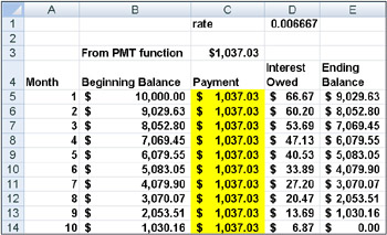
  Recall that in Chapter 10, “Circular References,” we found the monthly payment (assuming payments occur at the end of a month) on a 10-month loan for $8,000.00 at an annual interest rate of 10 percent to be $1,037.03. Could we have used Solver to determine our monthly payment? You’ll find the answer in the PMT By Solver worksheet in the file Finmathsolver.xlsx, which is shown in Figure 31-1.

  
  Figure 31-1: Solver model for calculating the monthly payment for a loan

• The key to our model is to use Equation 1 to track the monthly beginning balance. Our Solver target cell is to minimize our monthly payment. The changing cell is the monthly payment. The only constraint is that the ending balance in month 10 equal 0.

• I entered the beginning balance in cell B5. I entered a trial monthly payment in cell C5. Then I copied the monthly payment to the range C6:C14. Because we’ve assumed that the payments occur at the end of each month, interest is incurred on the balance at the beginning of the month. Our monthly interest rate (I’ve named cell C1 rate) is computed in D1 by dividing the annual rate of 0.08 by 12. The interest paid each month is computed by copying from cell D5 to D6:D14 the formula rate*B5. Each month, this formula computes the interest as .006666*(month’s beginning balance). By copying the formula (B5–(Payment–D5)) from cell E5 to E6:E14, we use Equation 1 to compute each month’s ending balance. Because (Month t+1 beginning balance)=(Month t ending balance), we compute each month’s beginning balance by copying from cell B6 to B7:B14 the formula =E5.

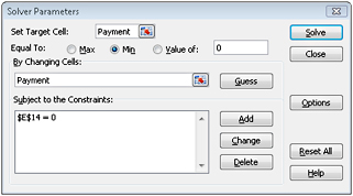
• We are now ready to use Solver to determine our monthly payment. To see how I’ve set up the Solver Parameters dialog box, take a look at Figure 31-2.

  
  Figure 31-2: Solver Parameters dialog box set up to determine mortgage payments

• Our goal is to minimize the monthly payment (cell C5). Note that the changing cell is the same as the target cell. The only constraint is that the ending balance for Month 10 must equal 0. Adding this constraint ensures that the loan is paid off. After we check the Assume Linear Model option and the Assume Non-Negative changing cells option (both located in the Solver Options dialog box; click Options in the Solver Parameters dialog box to select these options), the Solver calculates a payment of $1,037.03, which matches the amount calculated by the Excel PMT function.

• This model is linear because the target cell equals the changing cell and the constraint is created by adding multiples of changing cells.

• We should mention that when Solver models involve very large and/or very small numbers, the Solver sometimes thinks models that are linear are not linear. To avoid this problem, it is good practice to check the Use Automatic Scaling option in the Options dialog box. This should ensure that Solver properly recognizes linear models as being linear.

• Can I use Solver to determine how much money I need to save for retirement?

  By using Equation 2 (shown earlier in the chapter), we can easily determine how much money a person needs to save for retirement. Here’s an example.

• I am planning for my retirement, and at the beginning of this year and each of the next 39 years, I’m going to contribute some money to my retirement fund. Each year, I plan to increase my retirement contribution by $500. When I retire in 40 years, I plan to withdraw (at the beginning of each year) $100,000 per year for 20 years. I’ve made the following assumptions about the yields for my retirement investment portfolio:

  • During the first 20 years of my investing, the investments will earn 10 percent per year.

  • During all other years, my investments will earn 5 percent per year.

• I’ve assumed that all contributions and withdrawals occur at the beginning of the year. Given these assumptions, what is the least amount of money I can contribute this year and still have enough to make my retirement withdrawals?

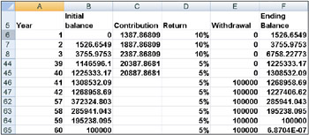
• You can find the solution to this question on the Retire worksheet in the file Finmath-solver.xlsx, shown in Figure 31-3 on the next page. Note that I’ve hidden many rows in the model.

  
  Figure 31-3: Retirement planning data that can be set up for analysis with Solver

• This worksheet simply tracks my retirement balance during each of the next 60 years. Each year, I earn the indicated interest rate on the retirement balance. I begin by entering a trial value for my Year 1 payment in cell C6. Copying the formula C6+500 from cell C7 to C8:C45 ensures that the retirement contribution increases by $500 per year during years 2–40. I’ve entered in column D the assumed return on my investments for each of the next 60 years. In cells E46:E65, I’ve entered the annual $100,000 withdrawal for years 41–60. Copying the formula (B6+C6–E6)*(1+D6) from F6 to F7:F65 uses Equation 2 to compute each year’s ending retirement account balance. Copying the formula =F6 from cell B7 to B8:B65 computes the beginning balance for years 2–60. Of course, the Year 1 initial balance is 0. We note that the 6.8704E-07 in cell F65 is approximately 0, with the difference due to roundoff error.

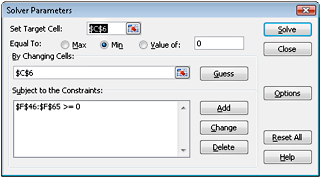
• The Solver Parameters dialog box for this model is shown in Figure 31-4. We want to minimize our Year 1 contribution (cell C6). The changing cell is also our Year 1 contribution (cell C6). We ensure that we never run out of money during retirement by adding the constraint F46:F65>=0. This formula ensures that the ending balance for Years 41–60 is non-negative.

  
  Figure 31-4: Solver Parameters dialog box set up for the retirement problem

• After checking the Assume Linear Model and Assume Non-Negative options in the Solver Options dialog box and clicking Solve in the Solver Parameters dialog box, we find that our first year’s contribution should equal $1,387.87.

• This model is linear because the target cell equals the changing cell and our constraint is created by adding multiples of changing cells. Note that because the return on the investments is not the same each year, there is no easy way to use Excel financial functions to solve this problem. Solver provides a general framework that can be used to analyze financial planning problems when mortgage rates or investment returns are not constant.