Designing the OLAP Structure

If youve followed our instructions to build a DW/BI system with surrogate keys, conformed dimensions, and well-managed dimension changes, then building an Analysis Services OLAP database is straightforward. There are several major steps:

1. Set up the design and development environment

2. Create a Data Source View

3. Create and fine-tune your dimensions

4. Run the Cube Wizard and edit the resulting cube

5. Deploy the database to your development server

6. Create calculations and other decorations

7. Iterate, iterate, iterate

Later in the chapter, we discuss physical storage issues, which are largely independent of the databases logical design.

Note 

Analysis Services contains features to help you overcome flaws in the design of the source database, like referential integrity violations, but were not going to talk about those features. Instead, build your DW/BI system correctly, as described in this book.

Getting Started

There are several steps in the setup process. First, you need to install and configure one or more Analysis Services development servers. You need to ensure the correct software is installed on developers desktops. You should have some clean data loaded into the data warehouse database, and you should have created a set of views on those database tables.

Setup

As the Analysis Services database developer, the only SQL Server components you must have on your desktop PC are the development tools, notably BI Studio and Management Studio. Many developers run the server components on their desktop PCs, but its not required. You can point to a shared Analysis Services development server, just as you would share a development relational database server.

Use BI Studio to design and develop the Analysis Services database, and Management Studio to operate and maintain that database. The way the tools have been broken apart may be confusing at first: After all, theres no such distinction for the relational database. With the appropriate permissions, you can enter DDL against a production relational database from within Management Studio. We all know thats a really stupid thing to do (although how many of us do it?). The new BI tools strongly discourage it for Analysis Services. From within Management Studio you can perform only the actions necessary to maintain the database: Add partitions, process partitions, backup, and so on. Any design change must occur within the BI Studio and be deployed into production. Deployment issues are discussed in Chapter 14. But when in doubt, remember: Use BI Development Studio for development, and use the Management Studio for management.

Analysis Services Tutorial

Work through the tutorial that ships with SQL Server 2005 before trying to design and build your first OLAP database. Its a good tutorial, and not only teaches you which buttons to push but also provides information about why. This chapter is not a replacement for the tutorial. Instead we assume youll learn the basics from the tutorial. Here, we focus more on process and advanced design issues.

Create Relational Views

In Chapter 4, we talked about creating a database view for each table in the dimensional model. End users and Analysis Services access to the relational database should come through the views. The views provide a layer of insulation, and can greatly simplify the process of making future changes to the DW/BI system. Give the views and columns user -friendly names: These names become Analysis Services object names like dimensions and attributes.

Tip 

Analysis Services does a pretty good job of turning the common styles of database object names into friendly names. It will parse CamelCase and Underscore_Case names, stripping underscores and inserting spaces as appropriate. Its not perfect; you do need to review the friendly names in the Data Source View.

The downside of using views is that you obscure any foreign key relationships defined in the data. Many tools automatically create join paths based on these relationships; these join paths must be added by hand when you use views. On the other hand, as we discuss in Chapter 4, its common to drop the foreign key relationship between fact and dimensions anyway.

Tip 

Creating the view layer sounds like make-work. But weve always regretted it when weve skipped this step.

Populate the Data Warehouse Database

You dont need to wait until the ETL system is finished, and the relational data warehouse fully populated with historical and incremental data, before you start working on the Analysis Services database. Technically, you dont have to populate the database at all. But thats just a theoretical point: In practice, you want to look at the data as youre designing the OLAP database.

Its helpful during the design process to work from a static copy of the warehouse database. Its much easier to design and debug the cube if the underlying data isnt changing from day to day. Most people fully populate the dimensions and several months of data in the large fact tables. Small fact tables, like the Exchange Rates fact table in the Adventure Works Cycles case study, can be fully populated.

Fully populate most of the dimensions because thats where most of the design work occurs. Dimensions are usually small enough that you can restructure and rebuild them many times, without an intolerable wait to see how the modified dimension looks. If you have a larger dimension, say 100,000 to 1 million members , you may want to work on a dimension subset for the early phases of the design cycle. Define your dimension table view with a WHERE clause so that it subsets the dimension to a reasonable size, iterate on the design until youre satisfied, and then redefine the view and rebuild the dimension at its full size . We can almost guarantee youll still tweak the design a few more times, but you should be past the worst of the iterations.

We mentioned that most people use a few months of fact data. This works great for structural design tasks like setting the grain, dimension usage, and base measures for that fact data. But defining complex calculations is often easier to do with a longer time series. As a simple example, consider a measure that compares sales this month to the same month last year.

If you have really big dimensions and facts, you should take the time to build a physical subset of the relational database. Keep all small dimensions intact, but subset large dimensions to less than 100,000 members. Randomly choose leaf nodes rather than choose a specific branch of the dimension. In other words, if you have 5 million customers, randomly choose 100,000 of them rather than choose all of the customers from California (who may not be representative of your full customer base). Choose the subset of facts from the intersection of your dimensions. Be very careful to avoid grabbing facts for the dimension members youve excluded from the test database. In other words, load facts for the 100,000 selected customers only.

Chapter 5 describes how to build a sandbox source system for developing the ETL system. That same subset, in the relational dimensional structure, may serve you again during Analysis Services design.

Tip 

Yes, this is a lot of work at a time when youre anxious to get started with Analysis Services. Youll be thankful later, when youre iterating on your cube design for the hundredth time. Also, this small database may be useful again for end user training.

Create a Project and a Data Source View

Finally, youre ready to use the tools to get started on the design process. Create an Analysis Services project in BI Studio, usually within the same solution as your Integration Services and Reporting Services projects.

Tip 

For those of you who would like to follow along as we create the Analysis Services database, first create the relational data warehouse database. You can download this database, MDWT_AdventureWorksDW, from the books web site, www.MsftDWToolkit.com .

By default, BI Studio points to the default instance on the local serverthe developers desktop. To specify a different Analysis Services instance or server, right-click on the project name in the Solution Explorer, and choose Properties. As illustrated in Figure 7.2, you can identify a server for development.

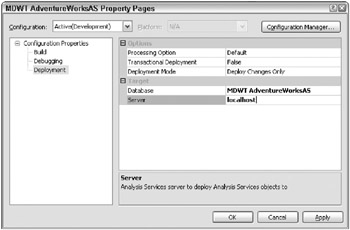
Figure 7.2: Deploy development projects to a different server

Tip 

Most DW/BI teams will use SQL Server Developer Edition, which contains all the functionality of Enterprise Edition. If youre using Standard Edition in production, change the Deployment Server Edition property of the project to Standard. That way, youll get warnings if you attempt to use functionality thats not available in Standard Edition.

The next step in designing the Analysis Services database is to create a Data Source View (DSV) on the relational data warehouse database. We introduced DSVs in Chapter 6, where they were optional. The Analysis Services database is built from the Data Source View, so you must create a DSV before designing the database.

Right-click on Data Source Views and choose New Data Source View. The Data Source Wizard prompts you to choose or create a Data Source. If your Analysis Services project is part of the same solution with your Integration Services or Reporting Services project, you should re-use the appropriate Data Source. Shared data sources are easier to manage in production because you have to go to only one place to change the characteristics of the connection.

STARTING THE ANALYSIS SERVICES SERVER

If youre running Analysis Services on your desktop computer, you may want to have the service start manually. Write a one-line batch file to start the service:

 net start MSSQLServerOLAPService 

Create a shortcut to this .bat file from your desktop. Create a similar command file to stop the service ( net stop MSSQLServerOLAPService ).

 

Tip 

Theres an option on the first screen of the Data Source Wizard to create a data source based on another object. Click this radio button to pick up the data source from another project rather than creating a new one.

Choose a subset of tables or views to include in the DSV. You can always add and delete tables from a DSV after its been built, so dont worry too much about getting the subset correct the first time through the wizard. The Select Tables and Views page of the Data Source View Wizard has a filter utility to make it easier to find the objects you want. Exclude any metadata tables, staging tables, or utility tables that you wont want in the cube you create.

Figure 7.3 illustrates the DSV for the MDWT_AdventureWorksDW database in the DSV Designer. The Properties pane for Customer is showing; notice that weve copied in the table description that we created in the Excel workbook way back in Chapter 3. Use the list of tables on the left-hand side to quickly find a table.

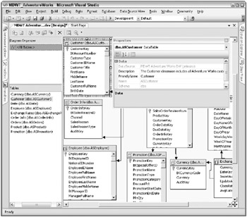
Figure 7.3: DSV for the MDWT_AdventureWorksDW database

Edit the DSV in the BI Studio DSV Designer. Within the schema pane of the DSV Designer, you can view the tables, columns, and relationships. You can also view the tables and columns in a tree view. The Diagram Organizer pane is useful for very complex DSVs. In it you can create subdiagrams for viewing smaller sets of tables.

Add tables (or views) and relationships to the DSV. You can change object names here, although your dimensional model should have friendly names already. When you create the Analysis Services database, it will take default names from these objects in the DSV. You can also add tables from the existing data source, or from additional databases and servers including non-SQL Server sources.

Warning 

Avoid using the DSV to cobble together an Analysis Services database from a variety of heterogeneous sources. First, unless youve scrubbed all the data, its not going to join well at all. Second, theres a considerable performance cost to joining remotely. Youre almost certainly better off cleaning and aligning the data and hosting it on a single physical server before building your cube. Yes: Youre better off building a data warehouse.

However, if youre careful and judicious, you can use this distributed sources feature to solve some knotty problems. A distributed DSV uses the SQL Server engine under the covers to resolve the distributed query. At least one SQL Server data source must be defined in order to create a distributed DSV.

You must construct the relationships correctly in the DSV because these relationships help define the Analysis Services database. A relationship between a fact and dimension table should appear, as in Figure 7.4. Make sure you set the relationship in the correct direction.

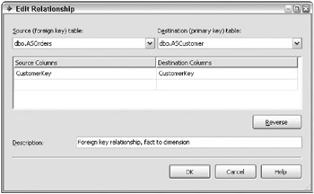
Figure 7.4: A Data Source View relationship between fact and dimension

The Description attribute for tables and columns in the DSV are picked up by the Cube Wizard and incorporated into the definitions of dimensions, attributes, and other cube objects. From there, most ad hoc query tools can show the descriptions to the business users. Youll run the Cube Wizard many times, so its really nice to get the descriptions populated in the DSV. Otherwise, the descriptions will get wiped out every time you re-run the Cube Wizard.

Dimension Designs

The database that you design and build in Analysis Services will be very similar to the relational data warehouse that youve built using the Kimball Method. This section describes how Analysis Services handles dimensions in general, and how it handles several of the dimension design issues we discussed in Chapter 3.

After weve talked about how OLAP dimensions correspond to the dimension tables in your relational data warehouse, we talk about the actual process of creating and editing those dimensions.

RUNNING THE CUBE WIZARD: THE ONE-CLICK CUBE

In most materials about Analysis Services 2005, including Books Online and the tutorials, youre encouraged to start building your OLAP database by running the Cube Wizard after youve defined the DSV. The Cube Wizard reads the relationships youve defined in your Data Source View, and automatically generates the definition for the entire OLAP database, including all dimensions.

Weve found that most people will take this route two or three times. It certainly makes a fun demo. But if youre trying to get work done, youll probably find an alternative process more productive. Create dimensions one at a time, as we describe in the next section. Work on each dimension, setting its attributes and properties correctly, processing and browsing it until you like the way it looks. Move down the list of dimensions until youve defined all the dimensions associated with a fact table. Only then should you run the Cube Wizard.

 

ANALYSIS SERVICES DIMENSION TERMINOLOGY

The terminology around dimensions in SQL Server 2005 Analysis Services is similar to the familiar Kimball Method terminology. Heres a brief list of vital Analysis Services vocabulary having to do with dimensions. These concepts are discussed in more detail later in this chapter. This sidebar introduces them so you can understand the vocabulary.

• Dimension: The concept is effectively identical to the Kimball Method usage of the term . In normal use, Analysis Services dimensions correspond exactly to a relational dimension. Some decorations are different, but the core concepts are the same.

• Attribute: An Analysis Services dimension attribute is directly analogous to a Kimball Method dimension attribute.

• Dimension hierarchy: A common drilldown path in the dimension, predefined by the system developer for the benefit of users.

  • Natural hierarchy: A drilldown path with referential integrity between attributes at different levels, like Year to Month to Day.

  • Navigation hierarchy: A drilldown path between unrelated attributes, like Gender to Age. This is sometimes called a reporting hierarchy .

    You wont find the terms natural hierarchy or navigation hierarchy in Books Online. But the distinction is very important for query performance, as well discuss in this chapter.

• Attribute hierarchy: Each dimension attribute is exposed as a single-level attribute hierarchy. You optionally define one or more multi-level dimension hierarchies from those attributes.

• Attribute relationship: An attribute relationship is, effectively, a declaration of referential integrity between two attributes. All attributes have an attribute relationship to the key of a dimension. You can and should define other attribute relationships.

• Member: A member is an item in a dimension level or attribute hierarchy. Examples are January 2006 in the Month level of the Date dimension, or Rural Cycle Emporium in the Customer level of the Customer dimension. A member is analogous to a row in the dimension table.

  • Leaf member: A leaf is a member at the finest grain of the hierarchy, like a date, customer, or employee.

  • All member: A member, usually defined only in Analysis Services, that represents the aggregation of all the leaf members: All customers, All products, and so on. The All member is optional.

  • Default member: The member thats included by default if a query does not reference the dimension. By default, the Default member is set equal to the All memberand behaves exactly as the relational database would if you exclude a dimension from the query.

• Many-to-many dimension: What the Kimball Method calls a multivalued dimension. A standard dimension has a one-to-many relationship between a dimension key and the fact table. A multivalued dimension has a many-to-many relationship. Common examples are patient hospital visits and diagnoses (one patient visit can have multiple diagnoses), and purchase reasons (a customer could have multiple reasons for purchasing your product). Multivalued or many-to-many dimensions are directly (and rather elegantly) supported in Analysis Services 2005.

• Parent-child hierarchy: What the Kimball Method calls a variable depth hierarchy. A variable depth hierarchy is characterized by a self referencing join. Canonical examples are an organizational hierarchy (employee to manager) or a bill of materials.

• Reference dimension: The Kimball Method doesnt have a name for this concept. A reference dimension is a dimension thats referenced by others. For example, many dimensions like Customer, Vendor, and Shipping Destination could all use the same Geography table. All you need is to put the Geography surrogate key into those primary dimensions. We havent found reference dimensions to be particularly useful, and we dont discuss them in this chapter.

• Fact dimension: A fact dimension is what the Kimball Method calls a degenerate dimension. Its a dimension thats populated from the fact table. The common example is a Purchase Order and Line Item Number from a sales transaction fact table. We dont expect users to slice and dice by PO numbers , but its often very convenient to have them available in both the relational data warehouse and the cube. However, we almost never build a separate relational dimension table from this kind of entity. Any interesting attributes of the purchase order have been pulled out into one or more dimension tables. This entity is halfway between fact and dimension, so we call it a degenerate dimension. There are several ways to support degenerate dimensions in Analysis Services.

 

Standard Dimensions

A standard dimension contains a surrogate key, one or more attributes and attribute hierarchies, and sometimes zero or more multi-level hierarchies. Analysis Services can build dimensions from dimension tables that:

• Are denormalized into a star structure, as the Kimball Method recommends

• Are normalized into a snowflake structure, with separate tables for each hierarchical level

• Include a mixture of normalized and denormalized structures

• Include a parent-child hierarchy

• Have all Type 1 (update history) attributes, Type 2 (track history) attributes, or a combination

Even though Analysis Services doesnt require a surrogate key, recall that surrogate keys are a cornerstone of the Kimball Method; build a permanent, enterprise Analysis Services database only from a dimensional relational source with surrogate keys.

Tip 

Analysis Services 2005 has built in many features to help you live without surrogate keys. For example, you can set up the database so that it automatically finds and fixes referential integrity violations. In our view, this activity should be done during the ETL process. Build Analysis Services databases from clean, dimensional data in the relational database.

Your business users will tell you whether dimension attributes should be tracked as Type 1 or Type 2. Weve found that most dimension attributes are tracked as Type 2. In Chapter 6 we talked extensively about how to set up your ETL process to manage the propagation and assignment of surrogate keys for Type 2 dimension attributes. Although Type 2 dimensions seem harder to manage in the ETL system, the payoff comes with your Analysis Services database. Analysis Services handles Type 2 attribute changes gracefully. The larger your data volumes , the more you should be relying on Type 2 changes, where they make sense for the business user.

Type 1 attributes can cause some problems for OLAP databases for the same reason theyre troubling in the relational world: pre-computed aggregations. When a dimension attribute is updated in place, any aggregations built on that attribute are invalidated. If you were managing aggregations in the relational database, youd have to write logic to fix the historical summary table when an attribute changes. Analysis Services faces the same problem. You dont have to do anything to fix up the historical attributesAnalysis Services does that for you. But this is an expensive operation. If you have a lot of Type 1 changes in a very large database, youre going to be unpleasantly surprised by the incremental processing performance. Later in this chapter we talk about some choices you can make in your design to minimize the cost of managing Type 1 dimension changes.

Variable Depth or Parent-Child Hierarchies

Variable depth or parent-child hierarchies are a useful way of expressing organization hierarchies and bill of materials explosions. However, as we discussed in Chapter 6, these dimension structures are difficult to maintain in the relational data warehouse. This is especially true if the dimension has Type 2 attributes.

If you can maintain your parent-child hierarchy in the relational database, either as a Type 1 or Type 2 dimension, then Analysis Services can consume it. Its straightforward to set up a Parent-Child dimension in Analysis Services. Its straightforward to query that dimensionfar more so in Analysis Services, by the way, than using standard SQL.

Tip 

Parent-child hierarchies are a valuable feature in Analysis Services. However, its not a trivial exercise to get them to perform well in a very large database, or with many members in the Parent-Child dimension. If your system is large, you may want to bring in an expert, or launch Phase 1 using a standard dimension. Add the parent-child relationship when your team has developed more expertise.

When you build a parent-child hierarchy in Analysis Services, you dont need a bridge table. You may have built a bridge table to facilitate relational queries, as described in Chapter 3. If so, you should eliminate that bridge table from the DSV for the Analysis Services database.

Multivalued or Many-to-Many Dimensions

The relational design for a multivalued dimension includes a bridge table between the fact and dimension tables. This bridge table identifies a group of dimension values that occur together. The example in the Adventure Works Cycles case study is the sales reason. Adventure Works Cycles collects multiple possible reasons for a customer purchasing our product, so each sale is associated with potentially many reasons. The bridge table lets you keep one row in the fact table for each sale, and relates that fact event to the multiple reasons.

This same structure serves to populate the Analysis Services database. The only nuance is that the bridge table is used as both a dimension table and a fact table, or as just a fact table, within Analysis Services. This seems odd at first, but it really is correct. The fact the bridge table tracks is the relationship between sales and sales reasonsyou could think of it as the Reasons Selected fact table.

Keep the bridge table from your relational data warehouse in your DSV. The designer wizards correctly identify the structure as a multivalued dimension, which Analysis Services calls a many-to-many dimension.

Creating and Editing Dimensions

Create dimensions one by one, by right-clicking on the Dimensions node in the Solution Explorer window and choosing New Dimension to launch the Dimension Wizard.

In the first screen of the Dimension Wizard, change the selection from the default choice of Create attributes and hierarchies . Instead, choose Create attributes only , as illustrated in Figure 7.5 . Weve never kept the hierarchies that the wizard recommends.

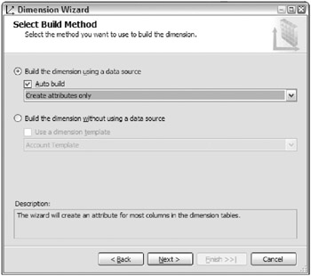
Figure 7.5: The Dimension Wizard: Select Build Method

BUILD THE DIMENSION WITHOUT USING A DATA SOURCE

You may be perplexed by the second major option: building a dimension without a data source. The Kimball Method, as you know from reading this book, moves the development project through a structured sequence, from requirements gathering to design, creating and populating the relational database, and then here to building the Analysis Services database. This option in the Dimension Wizard turns that sequence on its head, effectively jumping directly from the business requirements to the cube and dimension design. From there you create the relational data warehouse by auto-generating tables that exactly support the Analysis Services database design.

This is a good idea, as it keeps the designers focus on the business requirements rather than the existing data. However, it removes you too far from the data realities. When you go back to populate the relational data warehouse from the source systems, and browse the cube with data in it, youll probably find that youd prefer to restart the cube design from scratch.

This alternative path through the Dimension Wizard (and a similar path through the Cube Wizard) will have significant value in the future, assuming Microsoft develops a market in predefined BI templates. Several generic templates are shipped with Analysis Services, but the real value will come from a template closely targeted to a specific industrys business intelligence requirements and metrics. Even a very small consulting company, with expertise in a specific area, can build a template that will give you a huge head start for developing a shrink-wrapped or custom business intelligence application.

In the absence of good templates, this path through the wizard is most useful for prototyping, and as a learning aid. Consultants may use this feature for quickly building a proof of concept.

 

CONFORMED DIMENSIONS

People new to Analysis Services are often confused by the admittedly subtle distinction between a cube dimension and a database dimension. Dimensions are defined at the database level and shared across multiple fact tables. In the Dimension Designer, youre editing database dimensions.

Later, youll build a cube and associate dimensions with that cube. There are a handful of dimension properties that apply to the dimension in the cube. We wont discuss these properties until later in the chapter, when were discussing cubes. But keep this distinction between database dimensions and cube dimensions in the back of your mind.

 

After you choose the build method, the Dimension Wizard asks you to identify the main table for the dimension. On the bottom of this same screen of the wizard, you can identify a column to use as the member name. Usually you choose the business key here because users never want to see the data warehouse surrogate key. After this point, unless you have one of the unusual types of dimensions described in the previous section, you can usually accept all the defaults. Name the dimension, and click Finish.

BI Studio generates the metadata for the dimension and leaves you looking at the basic dimension structure in the Dimension Designer. Next, you need to edit your dimensions in the Dimension Designer, getting each dimension the way you like it before moving on to the next one. At this point in the process, you have only metadatathe definition of the dimension. Later we describe how you build, deploy, and process the dimension so you can actually look at the dimensions data.

Figure 7.6 shows the final version of the Product dimension. In the rightmost pane of the Dimension Designer is a representation of the tables or views that underlie the dimension. This pane is linked to the Data Source View; if you try to edit the entities in this pane, youre flipped over to the DSV Editor. When you edit the DSV and return to the Dimension Designer, the changes follow.

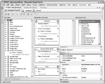
Figure 7.6: The Dimension Designer

The left-hand pane of the Dimension Designer is the Attributes pane, and shows the list of attributes within the dimension. Within the Attributes pane, you can rename and delete attributes, and change the properties of those attributes. To create a new attribute, drag a column from the data source in the DSV. You may need to create a calculated column in the DSV.

In the central pane of Figure 7.6 is the view of Hierarchies and Levels. Create a new hierarchy by dragging an attribute into the background area. Add levels to hierarchies by dragging and dropping.

The final pane in Figure 7.6 is the Properties pane, which is sometimes docked below the Solution Explorer. We set it to float in order to maximize screen real estate. Some of these properties are very important; others you might never change.

Figure 7.6 includes the properties of the Product dimension. If the Properties pane isnt showing, you can launch it by right-clicking on the Product dimension in the Attributes pane. In Figure 7.6 you can see that the Product dimension is highlighted, and the Properties pane title clarifies that youre looking at the dimensions properties. All the objects in the dimensioneach attribute, hierarchy, and levelalso have properties.

When youre editing a new dimension, take the following steps:

• Edit the names of the dimension and each attribute within the dimension.

• Edit the properties of the dimension.

• Edit the properties of each attribute.

• Create attribute relationships and edit their properties.

• Create hierarchies. Edit the hierarchies properties and the properties of each level.

• If necessary, define dimension translations.

• Build, deploy, and process the dimension so you can look at the dimensions data.

• Iterate, iterate, iterate.

The order of these steps isnt very important, but it helps to have a checklist. As you can see by reviewing the preceding list, the process of editing the dimension is largely a process of editing object properties. There are only a few other tasks, like creating attribute relationships and creating hierarchies.

In the next few sections, well run through the properties of dimensions, attributes, hierarchies, and levels. Well talk only about the most important properties that you can change; see Books Online for the details. In all cases, the Properties pane shows the properties for the highlighted item. Properties that youve changed from the default values are highlighted in boldface.

Editing Dimension Properties

A dimension has several editable properties. The most important are:

• Name: The name shows up in the user interface, so keep it short yet descriptive.

• Description: Most query tools for Analysis Services have a way of showing the description to the user, usually as a tool tip. As discussed previously, populate the Description metadata from the information you collected during your requirements gathering process.

• Type: Type is a frustratingly vague name for a property, but its hard to think of a better name. Type is a classification of the dimension thats used by Analysis Services only in a few special cases (Time and Account). Most of the time, if you set the dimension type to anything other than Time or Account, nothing happens. Set your Date dimensions Type to Time, so Analysis Services knows to use the dimension in time- related calculations.

  Tip 

  If youre a software developer building a packaged application on Analysis Services, you can use the dimension Type property to identify dimensions that are important to your application. The user can name the dimension whatever they want.

• AttributeAllMemberName: This label will show up to users when they start drilling down in the dimension and are looking at the All member of the dimension. By default, this property is blank, but that doesnt mean the All members name is blank. Instead, the default All member name is All (on English language systems).

• ErrorConfiguration: Analysis Services provides a lot of different options for handling problems with the dimension data, like duplicate keys and referential integrity violations. You can see the options if you set ErrorConfiguration to (custom). If youre sourcing your dimension from a solid Kimball Method dimension table, as weve described in great detail in this book, you shouldnt have to worry about this property. You shouldnt have bad dimension data; shame on you if you do.

  Tip 

  Though you shouldnt have duplicate surrogate keysor bad data anywhere in your dimensionits not unheard of between levels of a dimension hierarchy. For example, Postal Code should roll up to State, but in the source data there may be a handful of violations. If your ETL process doesnt catch and fix these violations, it should be modified to do so. If you change the ErrorConfiguration from its default to custom, and change the KeyDuplicate property from IgnoreError to ReportAndContinue or ReportAndStop, youll enlist Analysis Services help in figuring out where your data problems are. We usually turn on at least this level of error checking on dimensions.

• ProcessingMode: Sometimes, all of the aggregations associated with a dimension need to be recalculated. With this property, you can specify how quickly after an update the new cube data is available for users to query. We discuss this issue later in this chapter, in the section on Planning for Updates to Dimensions.

• ProactiveCaching: This property is useful for low latency population of the dimension. We discuss proactive caching in Chapter 17.

• StorageMode: Dimensions can be stored in Analysis Services format (MOLAP), or in the relational database (ROLAP). The vast majority of Analysis Services implementations should use MOLAP for all dimensions.

Reference 

See the Books Online topic Dimension Properties (SSAS) for a complete list and extremely brief description of all the dimension properties.

Editing Attribute Properties

As with the dimension properties, most of the important properties of an attribute are set correctly by the Dimension Wizard. A few useful properties arent set by the wizards. And if you add attributes within the Dimension Designer, you need to be aware of how to set these important attributes correctly.

• Name, Description, and Type: Ensure these properties are set correctly, as we discussed above for the dimension.

• Usage: This property is usually set correctly by the Dimension Wizard. One attribute for the dimension can and should have its usage set as Key. This is, obviously, the surrogate key for the dimension. Almost always, the other attributes are correctly set as Regular. The two exceptions are:

  • The parent key for a Parent-Child dimension (set to Parent)

  • A column in a Chart of Accounts dimension that defines the account type (set to AccountType)

• Source KeyColumns: By default, the KeyColumns property is correctly set to the appropriate column in the relational dimension table. The KeyColumns can be made up of more than one column, but in a Kimball Method system they always use the single-column surrogate key.

• NameColumn: You have an opportunity to set the NameColumn for the Key attribute in the Dimension Wizard. If you forgot to set it there, set it here. Users dont ever want to see the surrogate key; worst case, show them the business key. NameColumn is usually blank, unless you set it in the Dimension Wizard. Sometimes you set the NameColumn for other attributes of a dimension, especially levels that you will make into a natural hierarchy.

• OrderBy and OrderByAttribute: You can easily set an attribute to be ordered by either its key or its name. For example, we usually want to sort months not alphabetically (by month name), but by the month number. Occasionally, you want to sort one attribute not by its key or name, but by some other attribute in the dimension. To do this, you need to make the other attribute a Related Attribute of the first attribute, as we describe in the next section. Then you can set the sort order to that attribute. Alternatively, you could set AttributeHierarchyOrdered to False, in which case thered be no sort order at all.

• IsAggregatable: This property of an attribute specifies whether the attribute can be aggregated. It should almost always be set to the default value of True. If you set this property to False, the attribute hierarchy will not contain an All level.

• AttributeHierarchyDisplayFolder: You can add a lot of value to your Analysis Services database by adding display folders for the Attribute Hierarchies. If you have more than 10 to 12 attributes in your dimension, you should create multiple display folders and assign attributes to them. Creating a display folder is as simple as typing a name into the attributes AttributeHierarchyDisplayFolder property.

• AttributeHierarchyVisible: You can also prevent a specific attribute from appearing in the list of Attribute Hierarchies, by changing AttributeHierarchyVisible to False. Hiding the attribute hierarchy doesnt prevent you from exposing the attribute in a multi-level hierarchy. In fact, its common to hide the attribute hierarchy for attributes that are available through multi-level hierarchies, especially if the dimension has a lot of attributes.

ATTRIBUTE HIERARCHIES

Earlier in this chapter we noted that one of the biggest changes with Analysis Services 2005 is that dimensions are attribute-based rather than hierarchy-based. This is mostly a good thing because most dimension attributes, like Color , Size, and Cost, are not hierarchical.

With Analysis Services 2005, an Attribute Hierarchy is created by default for each attribute. Attribute Hierarchy isnt a great name for this object because its a flat hierarchy that consists only of the attribute and its All member. However, Attribute Hierarchies behave like, and show up in lists with, the multi-level hierarchies that you create for your users to navigate the dimension.

This improvement to Analysis Services, like most improvements, comes with a cost. The cost is reduced simplicity, both to the end user and to the developer. The end user now has to navigate many attributes rather than a few simple hierarchies. And the developer has to do whatever she canlike create Display Foldersto simplify the users view of what is, at its heart, a more flexible, and therefore more complicated database.

 

Tip 

The usefulness of the Display Folder depends on the client tool youre using to access the Analysis Services database. As we discuss in Chapter 13 , the Display Folder shows up in a Report Builder Report Model that you build atop the Analysis Services database. In this case, using Display Folders substantially improves the user experience.

• DefaultMember: Each Attribute Hierarchy has a default member. Unless you change it here, the default member is the All member for the dimension. This leads to the behavior youd expect: If youre not including an attribute in your query, you get all members just as a relational query would do. Occasionally, you might want to set the default member to something else. For example, in a Date dimension, you could set the default member for Year to the current year. You can even enter an MDX expression for the default member, if you really want to get fancy. But be warned ; you may end up confusing your users more than helping them.

• Parent-child properties: If the dimension has a parent-child hierarchy, you need to set up several properties. The most important one is the identification of the parent-child relationship. Just as one attribute in all dimensions is the key, in a Parent-Child dimension one attribute is identified as the Parent (set the Usage property to Parent for that attribute). The Dimension Wizard usually sets these properties correctly. You can look at the Employee dimension of the AdventureWorksAS sample database shipped with SQL Server for an example of a parent-child hierarchy. Other, less important, parent-child properties include:

  • RootMemberIf: How do you identify a member thats at the top of the tree? This would be the CEO in an employee hierarchy. There are several options, all self-explanatory.

  • NamingTemplate: How do you know what level of a parent-child hierarchy youre on? Many parent-child hierarchies dont have meaningful levels, but some doemployee organization is again a good example. For example, the top levels could be called Executive, VP, Senior Management, and then the remaining levels just called Level4, Level5, and so on. Use the NamingTemplate property to name these levels.

Reference 

See the Books Online topic Attribute Properties (SSAS) for a complete list of attribute properties, and a terse description of each property. There are many more attribute properties than weve listed here.

Related Attributes

Related Attributes is one of the most important characteristics of dimensions that youll need to edit. Related Attributes is the mechanism for declaring referential integrity between different attributes in a dimension. The declaration of attribute relationships is very important in the design of pre-computed aggregations and the Analysis Services indexes that are vital to query performance.

The only places to see this relationship in BI Studio are buried in the Attributes pane and Hierarchy pane of the Dimension Designer. Click on the plus sign next to an attribute to see its Related Attributes. (Dont ask the authors opinion of a user interface that hides such an important property!) When you create a dimension, the wizards automatically add all the dimensions attributes as Related Attributes of the key. This makes perfect sense: The key is unique, and all other attributes must by definition have a many-to-one relationship to it. Thus, all other attributes are Related Attributes of the key. The wizards also do a good job with snowflake dimension levels and the Date or Time dimension.

Create an attribute relationship by dragging an attribute from either the Attributes pane or the Hierarchy pane and dropping it under the attribute with which it has a one-to-many relationship. You can see some attribute relationships in Figure 7.6.

You should define Related Attributes between levels of a natural hierarchy. A great example that everyone understands is the Date dimension. All attributes are Related Attributes of the day, which is the grain of the Date dimension. Month is a Related Attribute of Day: Each day belongs to one and only one month. But Month is not a Related Attribute of Week: Each week may span multiple months. Quarter is a Related Attribute of Day and Month. Year is a Related Attribute of Day, Month, and Quarter.

Caution 

Indirect attribute relationships are preferred to direct attribute relationships. When you define an attribute relationship between two attributes, remove the relationship with the key, or any other attribute. In other words, when you make Year a related attribute of Month, you should remove it as a related attribute to Day. Month is still a related attribute of the key Day, and Year picks up that indirect relationship.

Lets suppose you just remembered that Quarter belongs between Month and Year. You add Year as a related attribute of Quarter, and Quarter as a related attribute of Month. As before, remove Quarter as a related attribute of Day. But also remove Year as a related attribute of Month.

This is really important for query performance. Its not even remotely obvious, nor is it well documented in Books Online.

The other important thing to remember about Related Attributes is that member keys must be unique, and defined to be unique. Returning to our Date dimension example, you would not want the Month attribute key to be January, February, and so on because these values are repeated each year. Even though theyre unique within the context of a hierarchytheres only one January each yearthey are not unique across the level. Instead, in this case, the correct key for the Month attribute is something that includes the year, like 200503.

Tip 

Add only the relationships that are truly many-to-one. Analysis Services sees an error if you define the relationship but the data violates that relationship. Unfortunately, Analysis Services by default will ignore that error. Sigh. A few pages back, in the section on Dimension Properties, we talked about changing the ErrorConfiguration setting. Its for exactly this reason that we like to change the dimensions KeyDuplicate error handling to ReportAndContinue or ReportAndStop.

By declaring Related Attributes correctly, youre informing Analysis Services that it can index and aggregate the data and rely on that relationship. Query performance will improve relative to a dimension whose Related Attributes are not set correctly. For medium and large data volumes, especially with very large dimensions, query performance improves substantially, largely because of improved design of aggregations that are based on the Related Attributes.

Theres a second reason for declaring Related Attributes correctly. This reason has to do with multiple fact tables at different levels of granularity: for example, quota data at a monthly level. In order to correctly define an Analysis Services database with data at different grains, the Related Attributes must be set properly. We talk about this issue again in the next section on hierarchies.

Warning 

Unless your OLAP database is tiny, its extremely important to set attribute relationships correctly.

There is one vital property associated with a Related Attribute: RelationshipType, which can be Rigid or Flexible. RelationshipType is where Analysis Services manages Type 1 and Type 2 dimension changes. Rigid means the relationship is fixed over time: The Related Attribute is managed as a Type 2 slowly changing attribute. Flexible means the relationship can change over time: The Related Attribute can be updated in place. As you might expect, Flexible is the default, and this setting works well and is easy to manage for small-to medium- sized cubes. The appropriate setting for this property is a business decision, but the choice has implications for cube load times. We talk about this issue later in the chapter, in the section on incremental cube processing.

If your cube is built on hundreds of gigabytes or terabytes of data, you need to pay careful attention to the settings for RelationshipType, and the aggregations that are built on attributes with flexible relationships. The issue, as we discuss later in the chapter, is about whether aggregations are dropped during incremental processing. Aggregations build really quickly, so this isnt a big deal for small cubes. But its an important tuning consideration for large cubes.

Reference 

See the Books Online topic Attribute Relationships (SSAS) for a description of attribute relationships.

See the Books Online topic Attribute Relationship Properties (SSAS) for a complete list of the properties of attribute relationships.

Check the Microsoft Project Real web site at www.microsoft.com/sql/bi/ProjectREAL for information about performance tuning Analysis Services databases.

Creating Hierarchies and Editing Hierarchy Properties

Creating hierarchies is incredibly easy. Just drag and drop attributes from the Attribute pane to the Hierarchies pane. You can create as many hierarchies as you want, or none at all.

As we mentioned previously in this chapter, multi-level hierarchies can be natural like Year, Month, Day. But a hierarchy doesnt have to be natural. You can create a hierarchy just for navigational or reporting purposes. In Figure 7.6 you can see a navigational hierarchy of Days to Manufacture and Safety Stock Level. Theres no relationship between the two attributes in this navigational hierarchy.

Weve just finished discussing attribute relationships without discussing hierarchies at length. But it should be clear that a natural hierarchy is one in which you canand shoulddefine attribute relationships between levels.

Hierarchies have few interesting properties:

• Name and Description: Ensure these properties are set correctly, as we discussed earlier for the dimension.

• AllMemberName: The name of the All member of the hierarchy. This property of the hierarchy is very much like the AttributeAllMemberName property of the dimension. All attribute hierarchies of a dimension share the same All Member name. User-defined hierarchies can have unique All Member names.

• DisplayFolder: Usually we want the hierarchy to show up in the top level when the user is browsing the dimension, so we leave DisplayFolder blank. If you have a really complicated dimension, it may make sense to put hierarchies into a display folder, as discussed earlier for attributes.

• Display order for hierarchies: A subtlety of the Dimension Designer interface is that the order in which the hierarchies are displayed in the hierarchy pane is the same order in which theyll appear in most query tools user interfaces. You can drag and drop the hierarchies to re-order them. This isnt an official property that you can edit, except by reordering the hierarchies.

Levels are constructed from attributes. Most of the interesting properties are associated with the underlying attribute, and you hardly ever have to change the properties of levels.

• Name and Description: Ensure these properties are set correctly, as we discussed earlier for the dimension.

• HideMemberIf: Usually, you want this property set to its default value of Never. You might want to hide a member if you have an unbalanced hierarchy that doesnt have members at all levels. The easiest example of an unbalanced hierarchy is a worldwide geography hierarchy. Small countries like Luxembourg dont have states, so youd usually just carry the country name down to the state level. In this case, you may choose to set HideMemberIf to ParentName or OnlyChildWithParentName. Be warned: Not all client query tools respect the HideMemberIf setting.

Reference 

See the Books Online topic Multilevel Hierarchy Properties (SSAS) for a complete list of the properties of a multilevel hierarchy.

See the Books Online topic Level Properties (SSAS) for a complete list of the properties of hierarchy levels.

Translations

Looking back to Figure 7.6, notice that there are three tabs at the top of the Dimension Designer. Weve been working in the Dimension Structure tab; the other two are Translations and Browser.

Translations are a very nice feature of Analysis Services 2005 Enterprise Edition. If your company is multinational, business users will probably prefer to view the cube in their native languages. A fully translated cube will have translations for its metadata (names of dimensions, attributes, hierarchies, and levels) as well as the dimension data itself (member names and attribute values). In other words, the dimension name Date needs to be translated, the attribute name Month, and the attribute values January, February, and so on.

The Translations tab is where you do this translation. You can add a new language by right-clicking in the window and choosing New Translation. Then you can type in the translations for the metadata.

If you want to translate the attribute values, your relational dimension table or view needs to have additional columns for the new languages. Typically, you remove these columns from the list of attributes in the Dimension Structure tab. The translations are populated from the source table rather than from attributes in the dimension.

The AdventureWorksAS database that ships with SQL Server has a good example of translations in the product dimension. Here, theyve chosen to translate only a few columns (Name, Category, and Subcategory); you can translate as many as you wish.

Browsing Dimension Data

The third tab across the top of the Dimension Designer is labeled Browser. This is where you can look at the dimensions data and hierarchies, as illustrated in Figure 7.7.

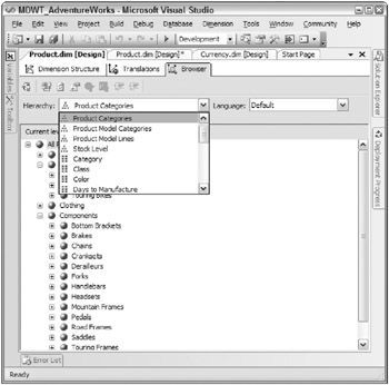
Figure 7.7: Browsing dimension data

Before you browse the dimensions data, you need to process the dimension. Up to now weve been dealing at the logical level, refining the dimensions structure without reference to its data.

Later in this chapter we talk more about building and deploying the Analysis Services database. But for the purposes of looking at a dimension whose attributes youve been editing, its sufficient to know that you dont need to build, deploy, and process the entire database in order to look at the dimension. You can right-click on the dimension in the Solution Explorer, and choose to build and deploy the changes to the project, then process the changed dimension.

Take time to look at the dimension in the browser. Look at the different hierarchies, available from the dropdown list as highlighted in Figure 7.7. If youve defined translations, you can view them here. Drill around the different levels and attributes in the dimension to ensure everything looks the way you want it to. Its a good bet that youll need to adjust something. On the first time through, youre fairly likely to have to go back to your ETL team and talk about improving the cleaning of the dimensions data. You should get detailed feedback from a representative of the business user community before you decide that a dimension is correctly defined.

Tip 

Its hard to overemphasize the importance of ensuring that the dimensions data and structure are clean and make sense to the business users. The dimension attributes are used for drilling down in queries; they also show up as report column and row headers. Spend time now to get them right, or youll be stuck with ugliness and confusion for years to come.

Keep working on your dimensions, hierarchies, and dimension data until youre pleased with them. Be sure to at least define the key level of each dimension correctly, before moving on to the Cube Designer.

Creating and Editing the Cube

After youve created and perfected your dimensions, its time to run the Cube Wizard to create the cube structure. The Cube Wizard looks a lot like the Dimension Wizard.

The Auto-Build feature of the Cube Wizard does an excellent job of reading the DSV and determining which tables are dimensions, which are fact tables, and which are bridge tables for many-to-many dimensions. You can examine the wizard page titled Identify Fact and Dimension Tables, but weve almost never found a mistaken identification. On the wizard page titled Review Shared Dimensions, specify that you want to use the existing dimensions, rather than have the Cube Wizard design new dimensions for you.

The next page of the wizard, Select Measures, offers an opportunity to review and rename the measures that will be created. You can edit and deselect measures here, or wait and do it in the Cube Designer. If the wizard finds dimensions in the DSV that you havent already created, it will list them and provide an opportunity to rename them on the Review New Dimensions page. When you finish with the Cube Wizard, youre dropped into the Cube Designer interface, illustrated in Figure 7.8. Anything you did in the Cube Wizard, you can do in the Cube Designer. You canand will!modify the objects that were created by the Cube Wizard. Use the Cube Designer to improve the cube, add new dimensions to a measure group, and add new measure groups.

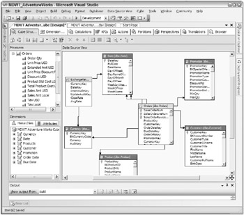
Figure 7.8: The Cube Designer

ANALYSIS SERVICES CUBE TERMINOLOGY

Earlier in this chapter we saw that Analysis Services terminology about dimensions is pretty similar to the Kimball Method terminology. The terminology around facts is quite different, although the concepts are roughly analogous. Here is a brief list of vital Analysis Services vocabulary having to do with facts and schemas:

• Measure: An Analysis Services measure is what the Kimball Method calls a fact.

  • Physical measures are defined from a column in the relational fact table view. Because youre sourcing from a view, you can create simple calculations in the view definition.

  • Calculated measures are defined using Multidimensional Expressions (MDX). We discuss this topic in much greater detail later in the chapter.

  • An aggregate function is associated with each measure. The default is to sum measures, but you can count, min, max, count distinct, or summarize by account. Some of the more complex aggregate functions, like by account, are available only in Enterprise Edition.

• Measure group: A measure group is directly analogous to a Kimball Method fact table. A measure group contains data at a grain specified by its dimensionality. If you have a relational fact table, you should expect to have a corresponding measure group.

• Cube: An Analysis Services cube is roughly analogous to a set of Kimball Method business process dimensional models. You could define a cube that encompasses the entire enterprise dimensional model, although that may be impractical for large and complex organizations.

  This definition of a cube differs from Analysis Services 2000. The best practice in Analysis Services 2005 is to define a single cube for a database. To those familiar with Analysis Services 2000, this would be like defining a virtual cube that logically combines all the physical cubes in a database. You are still permitted to create multiple cubes in a database, but you shouldnt. Instead, create a single cube with multiple measure groups.

• Analysis Services database: As discussed, an Analysis Services 2005 database should be one-for-one with the cube. Youre allowed to create multiple cubes within a single database, but the best practice is to create a database with a single cube. If you follow this practice, database and cube are synonymous.

• Perspective: Simplify the overall view of the cube by defining perspectives for different user communities. Perspectives are available only in SQL Server Enterprise Edition.

• Cells : A cell is a location in the cube.

  • A leaf cell is analogous to a row in a fact tablealthough more accurately its a column in a row.

  • A non-leaf cell is a location that corresponds to a summarized value, like Total Sales in November 2005 for Brand X. A cell is, effectively, the address of a number that you could bring back in a query. A cell represents a single coordinate from each dimension hierarchy, including the Measures dimension.

  • A cells contents can be calculated, as we discuss later in this chapter.

  • A cell can be empty. An empty cell takes up no space in an Analysis Services cube.

• Measure dimension: Analysis Services automatically creates a dimension called Measures where it stores all the fact-related attributes (called measures in Analysis Services). Users can locate measures by navigating to the Measures dimension.

 

Theres a lot going on in the Cube Designer, but its organized logically. Note the tabs going across the top of the window of Figure 7.8, titled Cube Structure, Dimension Usage, and so on. Well examine these tabs in greater depth, but first well quickly describe what each is for.

• Cube Structure: Use this view to examine the physical layout of the cubes sources. This is the active pane in Figure 7.8.

• Dimension Usage: Use this view to refine the dimensionality of each measure group.

• Calculations : Use this view to define, edit, and debug calculations for the cube.

• KPIs : Use this view to create and edit the Key Performance Indicators (KPIs) in a cube.

• Actions: Use this view to create and edit drillthrough and other actions for the cube. Actions are a powerful mechanism for building an actionable business intelligence application that does more than just view data.

• Partitions: Use this view to create and edit the partitions for a cube. Partitions are the unit of storage for cube data. You can specify different storage locations, storage modes, and refresh frequencies for different cube partitions. You can define different pre-computed aggregations for different partitions. Once a cube has been moved into production, you no longer edit partitions here. Instead, you manage partitions either from the Management Studio or your Integration Services packages.

• Perspectives: Use this view to create and edit the perspectives in a cube, to provide a simplified logical view of the cube for a set of business users.

• Translations: Use this view to create and edit the translated names for objects in a cube, like measure groups, measures, and calculations.

• Browser: Use this view to look at the data in the cube, once the cube has been deployed and processed .

Edit the Cube Structure

Figure 7.8 illustrates the Cube Structure tab of the Cube Designer. In the center pane is a representation of the Data Source View of the relational tables or views on which the cube is built. This is similar to the source data pane in the Dimension Designer, but a lot more complicated because it includes all the tables used in the cube. As with the Dimension Designer, if you want to edit the Data Source View youre flipped into the DSV Editor. Changes in the underlying DSV are reflected here immediately. In this view, fact tables are coded in yellow and dimensions in blue.

As with dimensions, the main activity in editing the cube structure consists of editing the properties of objects. In the case of the cube, edit the properties of measure groups, measures, and cube dimensions.

Edit Measure Groups and Measures

The small pane in the top left is where the cubes measure groups are listed. Open a measure group to see its measures. The most important properties for a measure group are:

• Name and Description: Ensure these are set correctly. Most Analysis Services client query tools reveal the Description as a tooltip.

• StorageMode and ProactiveCaching: Usually during development, these are set to MOLAP and Off respectively. We talk about these properties later in this chapter, when we discuss physical design considerations. Early in the development process, youll be iterating on the design. Using MOLAP storage noweven if later youll be moving to a different kind of storagekeeps the development cycle faster and simpler.

• StorageLocation: You can point the cubes MOLAP storage to a location other than the default.

We discuss the other properties of the measure group later, in the discussion of physical design considerations. For the initial iterations of the design and development, these settings are not very important.

The most important properties for a measure are:

• Name, Description, and FormatString: Ensure these are set correctly. Most Analysis Services client query tools automatically format data correctly, according to the FormatString.

• DisplayFolder: By default, measures are grouped by, well, measure group. Since each measure group can have dozens of measures, DisplayFolders give you an extra grouping layer within a measure group. They dont exist anywhere else. You make them up by typing them in the property window.

• AggregateFunction: Most measures are defined to summarize by summing or counting; less frequently by distinct count, min, or max. You can also define options for semi-additive or non-additive measures: averaging, beginning of period, end of period, and so on.

  Tip 

  You could set this behavior by right-clicking on the cube in the Solution Explorer and launching the Business Intelligence Wizard. The option to define semi-additive behavior sets the measures AggregateFunction.

• Visible: Its surprisingly common to hide a measure. Many measures are used for calculations but arent very interesting on their own. Hiding them reduces clutter for the business users.

Edit Dimensions in the Cube

The small pane in the lower left is where the cubes dimensions are listed. You can launch the Dimension Editor from here, or from the Solution Explorer as we discussed earlier.

The primary editing activity in the Dimensions pane of the Cube Structure tab is to add a new dimension or to re-order dimensions. The order of the dimensions in the cube, as they appear here in this pane, is the same as theyll show up to the users. Put the obscure dimensions at the bottom!

Tip 

There is a second implication of the order of the dimensions in this list, which is vital if you have complex calculations. The order of dimensions in this list affects the application of dimension calculations, like unary operators. This is particularly important for a financial model, where you might allocate along one dimension before calculating along a second dimension (usually the Account dimension). You can see this in the AdventureWorksAS database. The Organization dimension in that database must be listed before the Accounts dimension for the calculations to work properly. Try reordering the dimensions and recalculating the measure group to see how important the ordering is.

Dimensions are defined first at the database level, then optionally added to the cube. As we discussed earlier in the sidebar on cube terminology, the recommended practice is to have one cube in an Analysis Services database. This one cube contains multiple measure groups.

So, if you add new dimensions to your database after your initial run through the Cube Wizard, you may need to add them to your cube as well. Do so here.

The properties of a cube dimension that you might edit are:

• Name and Description: The dimension name as created in the database is usually the correct name. The only time youre likely to want to edit the name of the dimension in the cube is if the dimension has multiple roles. This is very common with the Date dimension: Order Date, Due Date, Ship Date, and so on are different roles of the Date dimension. Similarly, adjust the Description property for dimension roles.

You can also edit the properties of the hierarchy of a cube dimension, and attributes of a cube dimension. Its unlikely that youd want to do this.

Cube Properties

There are a few properties of the cube that you might want to adjust during development. You can see the list of these properties by clicking on the cube in either the Measures or Dimensions panes of the Cube Structure tab.

• Name and Description: Edit the cubes name and description as appropriate.

• DefaultMeasure: One measure will come up by default, if users dont specify a measure in a query. You should choose which measure that is, rather than letting Analysis Services choose it for you.

• StorageLocation: You can set the StorageLocation here, rather than for each measure group individually.

Most of the other options have to do with physical storage and processing, and are discussed later in the chapter. During the first part of the development cycle, the defaults are usually fine.

Edit Dimension Usage

You specify exactly how dimensions participate in measure groups on the next tab of the Cube Designer. Figure 7.9 illustrates the Dimension Usage tab for the MDWT_AdventureWorksAS sample cube. Our simplification of the Adventure Works schema presents a simple display. To see a more realistic display of dimension usage in a complex system, check out the AdventureWorksAS sample database that ships with SQL Server.

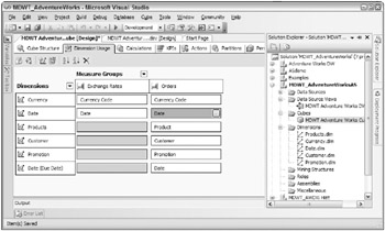
Figure 7.9: Dimension usage

The Dimension Usage tabs summarization of dimension usage is very similar to the Kimball Method bus matrix with the rows and columns flipped. At a glance you can identify which dimensions participate in which measure group, and at which cardinality.

The dimensionality of the Orders measure group displayed in Figure 7.9 has been modified from the defaults generated by the Cube Wizard. There are three date keys in the two fact tables, each with a different name. Originally, Analysis Services defined three roles for the Date dimension: Date from the Exchange Rates measure group, and Order Date and Due Date from the Orders measure group. However, the business users think of the Order Date as the main date key in the Orders table. Therefore, we deleted the Order Date role, and reassigned the OrderDateKey to the main Date role, using the Define Relationship window shown in Figure 7.10.

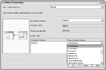
Figure 7.10: Editing dimension usage

Measure Groups at Different Granularity

Measure groups, and their underlying relational fact tables, may hook into a conformed dimension at a summary level. The most common scenario is for forecasts and quotas. Most businesses develop forecasts quarterly or monthly, even if they track sales on a daily basis. The fundamentals of dimensional modeling tell you to conform the Date dimension across uses, even if those uses are at different grains. By re-using the dimension, youre making it easy to compare quarterly data from multiple measure groups.

Analysis Services makes this conformation easy for you. All you have to do is correctly define the granularity attribute in the Define Relationship dialog box (set to DateKey in Figure 7.10). Make sure you set the Related Attributes properly in any dimension for which some measure groups join in above the grain.

Complex Relationships Between Dimensions and Measure Groups

There are several kinds of relationships between dimensions and measure groups, which you can set in the Dimension Usage tab. Most dimension relationships are Regular, but you can also specify Fact, Reference, Data Mining, and Many-to-Many relationships here.

The Cube Wizard does a good job of setting up these relationships correctly, but you should always check them.

Build, Deploy, and Process the Project

At this point in the development cycle, youve worked on your dimensions, and youve built and processed them several times. Youve defined the basic structure of your cube, including the relationships between measure groups and dimensions.

Now is a good time to perform the first processing of the OLAP database. The easiest way to do this is to right-click on the project name in the Solution Explorer, and choose Process. By choosing Process, youre doing three things:

• Building the project, looking for structural errors.

• Deploying that project to the target Analysis Services server, creating a new database structure (or updating an existing database structure).

• Processing that database, to fully or incrementally add data.

It makes sense to look at the data after processing has completed. See the discussion in the following section on the Browse Data tab.

THOSE PESKY ATTRIBUTE RELATIONSHIPS AGAIN

Its absolutely critical to set the Related Attributes properly in any dimension thats used at multiple granularities. You need to inform Analysis Services that it can expect referential integrity between various attributes in the dimension. If you arent careful here, you can see inconsistent query results because aggregations are computed and stored incorrectly, or will not show up at all.

Unfortunately, its easier to set up measure groups with different granularity wrong than it is to do it right. Review the Analysis Services tutorial topic Defining Dimension Granularity within a Measure Group before you develop your first summary measure group. And check your work (and the numbers) carefully .

 

Create Calculations

The third tab of the Cube Designer is where youll create calculations using the Multidimensional Expression language, or MDX. Most BI teams weve worked with have resisted learning MDX as long as they can. No one wants to learn a new language, but all eventually agree that at least one person on the team needs to step up to this challenge. The good news is that the BI Studio tools make it easy to define common calculations. And you can learn a lot about MDX by looking at how these calculations are defined for you.

You have opportunities to sprinkle MDX throughout the definition of the cube. The most obvious place is here, on the Calculations tab, where you can create calculated measures, other calculated members, sets, and calculated sub-cubes. Youll greatly improve the usefulness and user-friendliness of your Analysis Services database by defining common calculations that benefit all business users regardless of how theyre accessing the cube.

• Calculated measures will show up under the Measures dimension. Many calculated measures are quite simple, like the sum or ratio of two other measures. To a business user browsing the cube, calculated measures are largely indistinguishable from physical measures. Some query tools, including the Cube Browser integrated with BI Studio, will show a different icon for calculated measures and physical measures. A calculated measure is really just a calculated member, assigned to the Measures dimension. A very complex calculated measure may perform less well than a physical measure because calculations are performed at runtime.

• Calculated members can be created on any dimension. Non-measure calculated members can be very powerful. Theyre a way to create a kind of calculation that applies for some or all members. For example, you could create a calculated member Year To Date on the Date dimension, to automatically calculate multiple measures year-to-date.

  Tip 

  The Add Business Intelligence Wizard will create a wide variety of calculations for you, including the Year To Date calculated member.

• Named sets are a set of dimension members. A really simple named set would specify the set explicitly, perhaps as a list of important products. More complicated set definitions locate the set of products with a high price, products that sold well this year, and so on.

• Calculated sub-cubes are a way to calculate an arbitrary portion of the cubes data and summarizations. A common use of calculated subcubes is to allocate summary data (like monthly quotas) down to more fine-grained data. Or, calculated sub-cubes can provide a complex summarization method, if your business rules are more complicated than can be supported by the standard Aggregate Functions. If youre among the handful of people who are intimately familiar with calculated cells from Analysis Services 2000, youll dig into calculated subcubes and readily understand the improvements that MDX scripting and scoped assignments provide.

Tip 

How do you know whether you need a calculated member or a calculated sub-cube? A calculated member changes the visible structure of the cube; you can see the calculated member in the list of dimension members. A calculated sub-cube doesnt change the list of members or attributes in a dimension. Instead, it changes the way the numbers inside the cube are calculated.

The Calculations Tab

The Calculations tab of the Cube Designer is illustrated in Figure 7.11. As you can see, this is another complicated screen. But lets face it: Calculations are complicated.

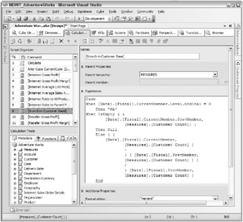
Figure 7.11: The Calculations tab

Tip 

In Figure 7.11 were illustrating the Calculations tab for the AdventureWorksAS database that ships with SQL Server, rather than our simplified version. Microsofts sample database contains a rich set of calculations, KPIs, and Actions. Exploring this database is an easy way to become familiar with using MDX to create calculated objects.

In the upper left is the Script Organizer. This pane lists the calculations that have been defined for this cube. The selected calculation is a calculated measure called [Growth in Customer Base], which calculates the change in the number of customers from one period to the next. The main area of the Calculations tab shows a form where this calculation is defined. The lower-left pane shows three tabs that contain a list of objects in the cube; a list of available functions, which you can drag into your calculation; and a set of templates, which can provide a starting point for some kinds of calculations.

This calculated member is defined on the Measures dimension; its a calculated measure. The next area contains the MDX for the calculation. Even without knowing anything about MDX, we probably can all parse this statement.

• If youre currently at the All Time levelif the level of the [Date].[Calendar Time] hierarchy is zeroyou want to display NA.

• If youre currently at the beginning of the datasetif there is no previous member of the Date dimensionyou want to display NULL.

• If youre anywhere in the Date dimension other than these two edge cases, you want to display the Customer Count for this period minus the Customer Count for last period, divided by the Customer Count for last period, in other words, the percentage change in the number of customers.

We could have illustrated a simpler calculated member in Figure 7.11, but this one has the advantage of being realistic. Its a nice example because it illustrates the important concept of defining your calculations relative to where the user is in the cube.

Note 

If youre defining lots of similar calculations, like [Annual Change for 2005] and [Annual Change for 2004], you should step back and figure out how to generalize. Probably you really need a single [Annual Change] calculation that computes relative to the current position in the cube: a far more elegant solution.

The calculation form also provides a place for you to add properties like formatting, color, and font. These properties can be conditional, which is particularly valuable for color: Display the measure in green if its positive, and red if its negative. You can also identify the Display Folder and Associated Measure Group for a calculation from within the Calculation Properties window.

Tip 

The Calculation Properties window is absurdly hard to find. Launch it by choosing Cube Calculation Properties, or click the Calculation Properties toolbar icon.

The calculation form view is a good way to create new measures and named sets. The form view is an item-by-item view of an underlying script. If you want to look at the entire script, switch to the script view by choosing Cube Show Calculations in Script (or click the Script toolbar icon).

Adding Business Intelligence

Unless youre already an MDX expert, one of the best places to get started in adding calculations to your cube is by using the Business Intelligence Wizard. This wizard will build for you the most common kinds of calculations. You can launch the Business Intelligence Wizard in several ways, including from the first icon on the Calculations toolbar.

Most applications will use the Business Intelligence Wizard to add time intelligence to their cube. This wizard option will automatically create for you calculations like [Year to Date], [12 Month Moving Average], and so on. These calculations appear on the Date dimension. Theyre non-measure calculated members. As such, they can apply to multiple underlying measures in one fell swoop.

A second advantage of the Business Intelligence Wizard is that you can pick apart the calculations to learn how they were done.

Define Key Performance Indicators

Key Performance Indicators (KPIs) are numbers or displays that are intended to measure the health of the organization. When KPIs are based on a clear understanding of the factors that drive the business, and a robust DW/BI platform, they can be an extremely powerful organizational management tool. Unfortunately, most KPIs are either brain-dead simple, divorced from the underlying data, or both. Really, who cares that sales are down 0.1 percent today unless we know that today is a Friday and Fridays sales are usually up 0.1 percent? And even if we did know the context, simply telling the executive that sales are down doesnt provide any understanding about why.

We hope that the definition and display of KPIs with Analysis Services will help address these shortcomings. The KPI implementation is well thought out. Because KPIs are defined in the cube, the supporting data can be made available in useful ways.

Analysis Services 2005 defines a KPI on the KPIs tab of the Cube Designer:

• Name of the KPI: And the measure group with which the KPI is associated.

• Value to be measured: The underlying measure for the KPI. Most often youll use a physical measure or a calculated measure that youve already defined. You can enter an MDX expression here, but it usually makes more sense to create a calculated measure and use that. In the very simple example we used in this section, the value to be measured might be [Sales Revenue].

Tip 

Whenever you specify an MDX expression when you create a KPI, the server will create a hidden calculated measure.

• Goal for the value: An MDX expression that defines the target for the measure. A trivial goal would be a number: The sales target is $100,000. That would give a stupid KPI. More interesting would be a goal to increase sales 0.1 percent from the same day the previous week, or a goal thats based on sales quotas

• Status: A graphic and an MDX expression that describe how the business is doing relative to its goal. Analysis Services provides several built-in graphic gauges, including thermometers, traffic lights, and happy faces. The MDX expression needs to evaluate to numbers between -1 (very bad) to +1 (very good). If youre clever about defining the status expression, you can do a good job of conveying important information about wide deviations from the goal, and keep minor deviations quiet.

• Trend: A graphic and an MDX expression that describe whether youre moving toward or away from your goal. Is the situation getting better or worse ? As with the status graphic, Analysis Services provides a few built-in trend graphics, notably a trend arrow. The MDX expression must evaluate to numbers between -1 (going south in a hurry) and +1 (getting better fast).

WHERE TO GO FOR HELP

Like so much weve introduced, Calculations and MDX are rich and complex topics about which entire books are written. Weve barely scratched the surface here.

The first place to go for help is the excellent section on Calculations in the SQL Server Analysis Services tutorial, which is part of Books Online. This tutorial walks you through the process of creating several calculated members, named sets, and calculated sub-cubes. The tutorial shows you how to debug your Calculation Script by setting breakpoints, stepping through calculations, and watching how each step modifies the cubes structure and data.

The debugger is a great feature. Learn how to use it, especially if you have any MDX scripts. The debugger is absolutely vital if you have multiple calculations that overlap one another.

The MDWT_AdventureWorksAS database is available on the books web site. It contains a handful of calculated members and sets, for the same simplified version of the AdventureWorks case study that weve used throughout this book.

The AdventureWorksAS database thats shipped with SQL Server is a good learning tool. It contains a lot of fairly complex calculations, especially for the finance module.

There are several books that the MDX expert on your team should own:

• MDX Solutions by Spofford, Harinath, Webb, and Civardi (Wiley, 2005). This is the new edition of the popular MDX Solutions edition for Analysis Services 2000. The new edition covers not only Analysis Services but also Hyperion Essbase, which now speaks MDX as well.

• Professional Analysis Services 2005 with MDX by Harinath and Quinn (Wrox, 2005). This book covers a lot more than MDX.

• Fast Track to MDX by Whitehorn, Pasumansky, and Zare (Springer, 2003). This introductory text was written for Analysis Services 2000, but it remains relevant for Analysis Services 2005. We expect it to be updated for 2005.

 

To display your KPIs, you need some client software that understands KPIs. An ad hoc query and reporting tool thats been designed to work well with Analysis Services 2005 will expose the KPI functionality. Your organization may have developed a reporting portal using Windows SharePoint Services, as discussed in Chapter 8. If so, you can embed KPIs in that portal by writing custom code to the APIs.

Widespread use of KPIs must wait until the client tool market matures, and especially until Microsoft releases new versions of information worker tools, like Excel and SharePoint, that are designed to work with Analysis Services 2005. Software vendors who are building packaged analytics on Analysis Services will probably be the first to use KPIs extensively in their front ends.

Create Actions

An Analysis Services Action is a command thats stored on the server. Actions are defined using MDX, which means that the command is context-sensitive. In other words, you can define an Action that executes when the user right-clicks on a cell in a report. The Action knows the values of each of the dimensions that make up the address of the cell and can execute a customized command for that address.

Like KPIs, the server-side definition of an Action is only half of the solution. You need a client tool that implements Actions. Its the job of the query tool to intercept the right-click on a report cell, and present (and execute) the appropriate list of Actions.

The most obvious use of an Action is to execute a relational query. As weve already described, the majority of SQL Server 2005 Analysis Services databases are built at the same grain as the underlying dimensional model. An interesting BI application could include an Action that drills back to enterprise data, perhaps even back to the original transaction system. This query Action can easily be implemented as an Action that launches a Reporting Services report.

Analysis Services provides for three kinds of Actions:

• Drillthrough to the cubes leaf-level data.

• Execute a Reporting Services report.

• Execute a generic Action. Actions can bring up a URL, return a rowset or dataset, or execute a command. An Action is defined as an MDX statement, and can be attached to specific parts of the cube. For example, you can have one Action that executes when someone right-clicks on the Month label in the Date dimension, and a second Action that launches when someone right-clicks on a data cell.

Tip 

Two kinds of ActionsHTML scripts and Command Line Actionspose security risks and should be avoided. Microsoft has moved these Action types out of the BI Studio interface. Youd have to create the Action by writing a script without the benefit of the UI.

Under the covers, the Drillthrough Action is simply a kind of rowset Action thats common enough that Microsoft built a simple user interface for defining it. Similarly, the Report Action is just an instance of a URL Action.

Drillthrough and Reporting Services Actions are very easy to set up. Generic Actions, like launching a parameterized web page, are pretty tricky. Start with something really simple, like launching a static web page (like Google or MSN). Add complexity a bit at a time. Process the cube and try out the Action in the browser window before adding another layer of complexity. If you change only an Action definition between processing, the processing step refreshes only metadata (not data), so processing occurs tolerably quickly.

Partitions

Use the Partitions tab of the Cube Designer to define the physical storage characteristics of your cube. During the first part of your development cycle, dont bother with this tab. Use the default settings so you can focus on getting the cube structure and calculations correct.

In the next section of this chapter, we discuss physical design considerations. We return to this tab and its settings, and talk at some length about whats going on under the covers, so you can make informed decisions about how to deploy your Analysis Services database in production.

Maintain Perspectives

Youll almost certainly define a few Perspectives if you follow the best practice recommendation of creating a single Analysis Services cube that contains multiple measure groups. Unless your implementation is really simple, this single-cube approach will lead to a structure thats challenging for business users to navigate.

An Analysis Services Perspective is like a big view on top of the database, limiting a users view to a set of related measure groups and dimensions. A Perspective is analogous to a business process dimensional model in the Kimball Method vocabulary. Its a very nice approach because youre not replicating data into multiple cubes: Youre simply providing different users with different views of the same data.

Use the Perspectives tab of the Cube Designer to define your cubes Perspectives. You can create as many Perspectives as you like; its a simple matter of choosing which portions of the overall cube to hide in each Perspective. You can also specify which measure is shown by default in each Perspective.

Most users will see only a few Perspectives, rather than the entire cube containing all measure groups. You can hide the cube itself, by setting its Visible property to False, and reveal only the Perspectives that contain the information your user communities are interested in.

It may feel as though Perspectives are a security mechanism. Not so! As we discuss in Chapter 12, Analysis Services security is applied at the database object level.

Unfortunately, Perspectives are not available in SQL Server 2005 Standard Edition. Many organizations dont have the users or data volumes needed to justify Enterprise Edition, but almost all organizations could benefit from Perspectives.

Define Translations

We introduced the notion of Analysis Services translations in the discussion of the Dimension Designer. This Translations tab in the Cube Designer is where you finish up the translating work. You can provide translations for the objects youve created in the Cube Designer: Display Folders, Measures, Cube Dimensions, Perspectives, KPIs, Actions, and Calculations.

When you use the Browser tab to browse the data, you can view the data with different Translations. This is fun to do, and if your organization is multilingual, it is certainly worth including in any demos you create for senior management. The AdventureWorksAS sample database that ships with SQL Server 2005 includes a rich set of translations.

The Translation feature works really well. It leverages the Localization technology in all Microsoft products. It picks up the locale ID from the users desktop and automatically displays either the appropriate translation, if it exists, or the default language. Most client tools dont need to do anything special.

Translations are not available in SQL Server 2005 Standard Edition.

Browse Data

The last tab of the Cube Designer is where you browse the data in the Analysis Services database. You dont need to work through all the other tabs before you take a look at the data. After youve defined the basic cube structure and verified the relationships with the dimensions, you generally want to check your work.

As we described earlier when talking about browsing the dimensions, you need to build, deploy, and process the cube before you can browse the data. The browser tab will remind you to do that if necessary.

Earlier in this chapter we talked about starting your Analysis Services development against a much reduced dataset. As you process the cube for the umpteenth time to check the implications of an edit, youll recognize why this was a good idea.