Physical Design Considerations

Up to this point in this chapter weve been discussing the logical design process for the Analysis Services OLAP database. Weve recommended that you work with a small subset of data so that you can concentrate on the structure, calculations, and other cube decorations, without worrying about the physical design.

CUBE PHYSICAL STORAGE TERMINOLOGY

Readers who are familiar with Analysis Services 2000 will already be familiar with most of the terminology for the physical storage and processing of the Analysis Services database. This sidebar merely defines these concepts. Recommendations and implications are discussed in detail elsewhere in the chapter.

• Leaf data: Leaf data is the finest grain of data thats defined in the cubes measure group . Usually, the leaf data corresponds exactly to the fact table from which a cubes measure group is sourced. Occasionally youll define a measure group at a higher grain than the underlying fact table, for example by eliminating a dimension from the measure group.

• Aggregations: Pre-computed aggregations are analogous to summary tables in the relational database. You can think of them as a big SELECT GROUP BY statement whose result set is stored for rapid access.

• Data storage mode: Analysis Services supports three kinds of storage for data.

  • MOLAP: Leaf data and aggregations are stored in Analysis Services MOLAP format.

  • HOLAP: Leaf data is stored in the relational database, and aggregations are stored in MOLAP format.

  • ROLAP: Leaf data and aggregations are stored in the source relational database.

• Dimension storage mode: Dimension data, corresponding to the relational dimension tables, can be stored in MOLAP format or left in the relational database (ROLAP mode).

• Partition: Fact data can be divided into partitions. Most systems that partition their data do so along the Date dimension; for example, one partition for each month or year. You can partition along any dimension, or along multiple dimensions. The partition is the unit of work for fact processing. Partitions are a feature of SQL Server Enterprise Edition.

• Fact processing: Analysis Services supports several kinds of fact processing for a partition.

  • Full processing: All the data for the partition is pulled from the source system into the Analysis Services engine, and written in MOLAP format if requested . Aggregations are computed and stored in MOLAP format if requested, or back in the RDBMS (ROLAP mode).

  • Incremental processing: New data for the partition is pulled from the source system and stored in MOLAP if requested. Aggregationseither MOLAP or ROLAPare updated. Its your job to tell Analysis Services how to identify new data.

• Proactive caching: Proactive caching is an important new concept for Analysis Services 2005. Its particularly interesting for low latency databasesfor populating the cube in real time (or near real time). When you set up proactive caching, youre asking Analysis Services to monitor the relational source for the measure groups partition and to automatically perform incremental processing when it sees changes.

 

Now its time to start addressing the physical issues. Most of the time, physical implementation decisions are made independently of the logical design. Thats not completely true, and in this section we discuss how some design decisions can have a large impact on the manageability and performance of your cube.

Storage Mode: MOLAP, HOLAP, ROLAP

The first question to resolve in your physical design is the easiest one. Should you use MOLAP, HOLAP, or ROLAP mode to store your Analysis Services data? The answer is MOLAP.

Were not even being particularly facetious with this terse answer, but we will justify it a bit.

Analysis Services MOLAP format has been designed to hold dimensional data. It uses sophisticated compression and indexing technologies to deliver excellent query performance. All else being equal, query performance against a MOLAP store is significantly faster than against a HOLAP or ROLAP store.

Some people argue that MOLAP storage wastes disk space. Youve already copied data at least once to store it in the relational data warehouse. Now youre talking about copying it again for the cube storage. To this argument we reply that a relational index also copies data. No one asserts you shouldnt index your relational database.

MOLAP storage is highly efficient. The leaf data in MOLAP mode (data and indexes) tends to require about 20 percent of the storage of the relational source (data only, no indexes). The MOLAP store of the leaf data is comparable in size to a single relational index on the fact tableand buys a lot more for you than any single relational index could possibly do.

Another common argument against MOLAP is that it slows processing. ROLAP is always the slowest to process because writing the aggregations to the relational database is expensive. HOLAP is slightly faster to process than MOLAP, but the difference is surprisingly small.

Dimensions also can be stored in MOLAP or ROLAP mode. Use MOLAP.

Note 

Why does Microsoft offer these alternative storage modes, if theyre inferior to MOLAP storage? The main answer is marketing: Its been an effective strategy to get Analysis Services into companies that would never countenance an instance of the SQL Server relational database in their data center. The multiple storage modes make the initial sale. Often, the DW/BI team figures out how much faster MOLAP is, and convinces management that its okay. Its also a hedge against the future. Its possible that improvements to relational technology could make HOLAP or ROLAP storage more appealing. Certainly wed love to see Analysis Services indexing, aggregation, compression, and processing abilities integrated into the SQL Server RDBMS, although we dont think thats particularly likely in the near future.

In Chapter 17 we back off slightly from the strong recommendation to use MOLAP. If you have a compelling business need for near-zero data latency from the cube, you may set up a ROLAP partition for data for the current hour or day.

Designing Aggregations

The design goal for aggregations is to minimize the number of aggregations while maximizing their effectiveness. You dont have to define every possible aggregation. At query time, Analysis Services will automatically choose the most appropriate (smallest) aggregation that can be used to answer the query. Aggregation design is a difficult problem, and Analysis Services provides several tools to help you out.

Before we talk about designing aggregations, however, its worth pointing out that very small cubes dont really need aggregations at all. During your development cycle, youre probably working with a small enough dataset that you dont need to worry about aggregations. Systems with small data volumes may not need to create any aggregations even in production. If you have only a hundred thousand rows in your measure groups partition, you dont need to worry about aggregations. Even large enterprises can find that many of their measure groupsfor example for quotas and financial dataare so small that aggregations are unnecessary.

Large data volumes, of course, do require thoughtful aggregation design. You should be experimenting with different aggregation plans in the later part of your development cycle, when you start to work with realistic data volumes. During development, you can design aggregations with the BI Studio, by launching the Aggregation Design Wizard from the Partitions tab of the Cube Designer. Figure 7.12 shows the Aggregation Design Wizard.

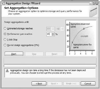
Figure 7.12: The Aggregation Design Wizard

In the Partitions tab you can see the partitions in each measure group. Launch the Aggregation Design Wizard displayed in Figure 7.12 by clicking on the Aggregations column for the partition.

The Aggregation Design Wizard will design aggregations based on the cardinality of your data. It looks at your dimensions and figures out where aggregations are going to do the most good. As a simplification of what its doing, consider that aggregating data from a daily grain up to monthly creates an aggregation thats one-thirtieth the size of the original data. (This isnt strictly true, but suffices for explanatory purposes.) But summarizing from monthly to quarterly gives an aggregation thats one-fourth the size. The Aggregation Design Wizard has reasonably sophisticated algorithms to look at the intersection of hierarchical levels to figure out where aggregations are best built.

We recommend that you use the Aggregation Design Wizard during development. Set the performance gain reaches number very low: 5 to 20 percent, as illustrated in Figure 7.12.

Tip 

One of the most common physical design mistakes is to build too many aggregations. The Aggregation Design Wizard positively encourages you to build too many aggregations, with its default setting of 30 percent. The first several aggregations provide a lot of benefit. After that, the incremental benefit at query time is slight ; and the cost during processing time can grow substantially.

As clever as the Aggregation Design Wizard is, and as good as its recommendations are, its missing the most important information in aggregation design: usage. The aggregations that you really want are those based on the queries that business users issue.

At the end of the development cycle, and as you move your Analysis Services database into the testing process, you should have developed the common queries and reports, as described in Chapters 8 and 9. Even in a test environment, running these common queries and reports against the database will provide much better information for aggregation design than the Aggregation Design Wizard uses.

We discuss how to develop a plan for ongoing tuning of usage based aggregations in Chapter 15. For the time being, remember to use the Aggregation Wizard during development, if your data is big enough to need aggregations. Plan to use usage-based aggregations in production.

Partitioning Plan

You can define multiple partitions for a measure group. Multiple partitions are a feature of SQL Server Enterprise Edition, and are very important for good query and processing performance for large Analysis Services measure groups. If you have a measure group with more than 50 million rows, you really should be using partitioning.

Partitioning is vital for large measure groups because partitions can greatly help query performance. The Analysis Services query engine can selectively query partitions: Its smart enough to access only the partitions that contain the data requested in a query. This difference can be substantial for a cube built on, say, a billion rows of data.

The second reason partitioning is valuable is for management of a large cube. Its faster to add a days worth of fact data to a small partition than to incrementally process that same day of data into a huge partition that contains all of history. With a small partition for current data, you have many more options to easily support real-time data delivery.

Partitioning also makes it possibleeven easy!to set up your measure group to support a rolling window of data. For example, your users may want to keep only 90 days of detailed data live in the cube. With a partitioned measure group, you simply drop the dated partitions. With a single partition, you have no option for deleting data other than reprocessing the entire measure group.

Partitioning improves processing performance, especially for full processing of the measure group. Analysis Services automatically processes partitions in parallel.

The largest measure groups, containing hundreds of millions or even billions of rows, should be partitioned along multiple dimensions: say by Month and Product Group. More partitions are better for both query and processing performance, but at the cost of making your maintenance application more complicated.

Tip 

If youve defined a lot of partitions, say a thousand, Management Studio will be slow. Itll take a few minutes to populate the lists of database objects.

You can always set up partitioning on your development server because SQL Server Developer Edition contains all the functionality in Enterprise Edition. But those partitions wont work on your production server if you use Standard Edition in production. As we described previously in this chapter, be sure to set the projects Deployment Server Edition property, so Analysis Services can help you avoid features that wont work in production.

Set up the initial partitioning plan in BI Studio, from the Partitions tab. Figure 7.13 illustrates the Partitions tab, this time for multiple partitions of the Orders measure group. The Orders measure group is partitioned by half- years . The first partition should always be empty; its been defined to hold all data before the first row that exists in the source system. Each subsequent partition is defined to select only the rows for contiguous six month blocks. The source query for one partition is shown. Analysis Services automatically generates most of the query. You need simply add the WHERE clause.

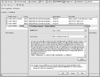
Figure 7.13: The Partitions tab and the partition source definition

Tip 

You need to be very careful to define the WHERE clauses correctly. Analysis Services isnt smart enough to see whether youve skipped data or, even worse , double-counted it.

There are several critical pieces of information to set correctly whenever you create a new partition:

• Source: Its your job to ensure that the data that flows into each partition doesnt overlap. In other words, the partition for year 2005 needs a source query that limits its data only to 2005.

• Slice: The Slice is where you tell Analysis Services which partitions to selectively access when resolving a query. Analysis Services 2005 sets this property automatically for you for MOLAP partitions. If you have a ROLAP partitionwhich is relatively unlikely unless you have a very low latency partitionset the slice by hand.

• Aggregations and storage: One interesting feature of Analysis Services partitions is that storage mode and aggregation design can differ for each partition. The most common intentional use of this feature is to add new kinds of aggregations only to current partitions as the aggregation plan changes over time.

When youre working with your database in development, you set up the partitions by hand in BI Studio. In test and production, you need to automate the process of creating a new partition and setting its source and slice. These issues are discussed in Chapter 15.

Planning for Deployment

After youve developed the logical structure of your Analysis Services database using a subset of data, you need to process the full historical dataset. This is unlikely to take place on the development server, unless your data volumes are quite small. Instead, youll probably perform full cube processing only on the test or production servers.

In Chapter 4, we discussed some of the issues around where the Analysis Services data should be placed. We discussed using RAID and SAN arrays; you should have your hardware vendor assist with the detailed configuration of these technologies.

One of the biggest questions, of course, is how to size the system. Earlier in this chapter we mentioned the 20 percent rule: The leaf level MOLAP data tends to take 20 percent of the space required by the same data in the relational database (data only, no indexes). Another equally broad rule of thumb is that aggregations double that figure, up to a total of 40 percent of the relational data. This is still amazingly small.

Tip 

Weve seen only one or two cubes whose leaf data plus aggregations take up more space than the relational data (data only, no indexes). That doesnt mean its not possible, but it is a reasonable upper bound to consider during the early stages of planning.

Your system administrators, reasonably enough, want a more accurate number than this 40 percent figure pulled from the air. We wish we could provide you with a sizing tool, but we dont know how to solve that problem. Exact cube size depends on your logical design, data volumes, and aggregation plan. In practice, the way people perform system sizing for large Analysis Services databases is to process the dimensions and one or two partitions using the initial aggregation plan. The full system data requirements scale up the partitions linearly (ignoring the dimension storage, which usually rounds to zero in comparison to the partitions).

Historical Processing Plan

In an ideal world, youll fully process a measure group only once, when you first move it into test and then production. But change is inevitable, and its pretty likely that one or more necessary changes to the databases structure will require full reprocessing.

You can fully process a measure group from within Management Studio: right-click on the measure group and choose Process. Once youre in production, this is not the best strategy for full processing. Instead, you should write a script or Integration Services package to perform the processing.

Tip 

Dont get in the habit of using Management Studio to launch processing. This isnt because of performanceexactly the same thing happens whether you use Management Studio, a script, or Integration Services. The difference is in a commitment to an automated and hands-off production environment. These issues are discussed in Chapter 15 .

You can create the basic processing script from the Management Studio Process Measure Group dialog by choosing the Script option. This option generates a script that you can execute in Management Studio, or use the Integration Services Execute Analysis Services DDL task.

We recommend that you use an Integration Services package rather than a script to perform measure group processing. This is especially true if youre using Integration Services for your ETL system, as youll have a logging and auditing infrastructure in place. Integration Services includes a task to perform Analysis Services processing. A sample package for fully processing the MDWT_AdventureWorksAS database is included on the books web site.

Incremental Processing Plan

Long before you put your Analysis Services database into production, you need to develop a plan for keeping it up-to-date. There are several ways to do this. Scheduled processing will continue to be the most common method of processing. Analysis Services 2005 offers a new processing method called Proactive Caching. Proactive caching is tremendously important and interesting for real-time business intelligence, and we discuss it in some length in Chapter 17.

You can also populate a cube directly from the Integration Services pipeline, without first storing it in a relational table. This is an interesting concept, especially if you multicast the flow to populate the cube and relational data warehouse at the same time. However, most mainstream applications will first store the data in a relational data warehouse.

Scheduled Processing

Scheduled processing of Analysis Services objects is basically a pull method of getting data into the cube. On a schedule, or upon successful completion of an event like a successful load, launch a job to pull the data into the cube. In this section were providing an overview of techniques. We go into greater detail in Chapter 15.

Full Reprocessing

The simplest strategy is to perform full processing every time you want to add data. Were surprised by how many people choose this strategy, which is akin to fully reloading the data warehouse on every load cycle. Its certainly the easiest strategy to implement. Analysis Services performs processing efficiently , so this approach can perform tolerably well for monthly or weekly load cyclesor even daily for very small measure groups.

The same script or Integration Services package that you used for the initial population of the cube can be re-executed every week or month.

Incremental Processing

If your data volumes are large enough that full processing is not desirable, the next obvious choice is to schedule incremental processing.

Incremental dimension processing is straightforward and can be scripted in the same way as database, cube, or measure group full processing. In Chapter 6, we recommend that you create an Integration Services package for each dimension table. You can add the Analysis Services processing task to each dimensions package, to automatically start dimension processing when the corresponding relational dimension has successfully loaded. Alternatively, wait until the relational work is done and process all Analysis Services objects together in a single transaction.

Incremental measure group processing is more complicated than dimension processing because you must design your system so you process only new data. Analysis Services doesnt check to make sure youre not inadvertently adding data twice or skipping a set of data.

The best way to identify the incremental rows to be processed is to tag all fact table rows with an audit key, as we describe in Chapter 6. All rows that were added today (or this hour, or this month) are tied together by the audit key. Now, you just need to tell Analysis Services which batch to load. You could write a simple program that would redefine a view of the fact table that filters to the current batch. Or, define a static metadata-driven view definition that points Analysis Services to the fact rows that havent been loaded yet.

Tip 

Its tempting to use the transaction date as the filter condition for the view or query that finds the current rows. In the real world, we usually see data flowing in for multiple days, so we tend to prefer the audit key method. If youre sure that cant happen in your environment, you can use the transaction date.

As before, once your view of the fact table has been redefined (if necessary) to filter only the new rows, its simple to launch measure group processing from a script or package.

Incremental Processing with Multiple Partitions

If youre using SQL Server Enterprise Edition and are partitioning your measure groups, your incremental processing job is even more challenging. First, you need to be sure that you create a new partition or partition set before you need it. In other words, if youre partitioning your measure group by month, then each month you need to create a new partition designed to hold the new months data.

Tip 

Theres no harm in creating twelve monthly partitions in advance. But you still need to add some logic to your Integration Services package, to be sure you march through the partitions as each new month begins.

Make sure that the source query for the measure groups incremental processing has two filters:

• Grab only the rows that are new.

• Grab only the rows that belong in this partition.

This is particularly tedious if you have late-arriving factsin other words, if todays load can include data for transactions that occurred a long time ago. If this is the case, youll need to set up a more complicated Integration Services package. Query the data loaded today to find out which partitions youll need to incrementally process; define a loop over those time periods.

Reference 

SQL Server includes a sample Integration Services package that manages Analysis Services partitions. Explore and leverage this excellent sample. Its installed by default at C:\Program Files\Microsoft SQL Server\90\Samples\Integration Services\Package Samples\SyncAdvWorksPartitions Sample.

Planning for Updates to Dimensions

Updates to dimensions generally happen gracefully and automatically in the dimension incremental processing. The easiest kind of dimension update is a Type 2 dimension change. Analysis Services treats a Type 2 change as a new dimension member: It has its own key, which the database has never seen before. From the point of view of dimension processing, theres no way to distinguish between a new set of attributes for an existing customer and a new row for a new customer.

Type 1 changes are picked up during dimension processing. Type 1 changes are potentially expensive because if any aggregation is defined on the Type 1 attribute, that aggregation must be rebuilt. Analysis Services drops the entire affected aggregation, but it can re-compute it as a background process.

Specify whether or not to compute aggregations in the background by setting the ProcessingMode property of the dimension. The ProcessingMode can be:

• Regular: During processing, the leaf-level data plus any aggregations and indexes are computed before the processed cube is published to users.

• LazyAggregations: Aggregations and indexes are computed in the background, and new data is made available to the users as soon as the leaflevel data is processed. This sounds great, but it can be problematic for query performance, depending on the timing of the processing. You want to avoid a situation where many users are querying a large cube at a time when that cube has no indexes or aggregations in place because its performing background processing.

For many applications, use lazy aggregations, and choose the processing option on the dimension to Process Affected Objects. This processing option ensures that indexes and aggregations are rebuilt as part of the incremental processing transaction.

The place to worry about a Type 1 change is if you have declared the attribute to have a rigid relationship with another attribute: in other words, if you have declared there will never be a Type 1 change on the attribute. You do want to use rigid attribute relationships because they provide substantial processing performance benefits. But if you try to change the attribute, Analysis Services will raise an error.

Deleting a dimension member is impossible , short of fully reprocessing the dimension. Fully reprocessing a dimension requires that any cubes using this dimension also be fully reprocessed. If you must delete dimension members, the best approach is to create a Type 1 attribute to flag whether the dimension member is currently active, and to filter those dimension members out of most reports and queries. Monthly or annually, fully reprocess the database.

Planning for Fact Updates and Deletes

The best source for an Analysis Services cube is a ledgered fact table. A ledgered fact table handles updates to facts by creating an offsetting transaction to zero out the original fact, then inserting a corrected fact row. This ledgering works smoothly for the associated Analysis Services measure group, because the ledger entries are treated as new facts.

Sometimes its not that easy. How do you plan for the situation where you mess up and somehow mis-assign a bunch of facts to the wrong dimension member? The only solutionunless you want to ledger out the affected rowsis to fully reprocess the affected partition.

Tip 

Multiple partitions are starting to sound like a really good idea.

There are several kinds of deleted data. The simplest, where you roll off the oldest month or year of fact data, is easily handled with a partitioned measure group. Just delete the partition by right-clicking it and choosing Delete in Management Studio or, more professionally, by scripting that action.

As with fact updates, deleting specific fact rows is impossible. The scenario is fairly common: You inadvertently load the same data twice into the relational database. Its unpleasant but certainly possible to back out that load from the relational tables, especially if you use the auditing system described in Chapter 6. But within Analysis Services, youre pretty much out of luck: Fully reprocess the affected partition.

Tip 

As we describe in Chapter 6 , your ETL system should perform reasonableness checks to ensure youre not double-loading. If you have late-arriving facts, where youre writing data to multiple partitions during each days load, youll be especially motivated to develop a solid ETL system.