Details

Proximity Measures

The following notation is used in this section:

v	the number of variables or the dimensionality
x j	data for observation x and the j th variable, where j = 1 to v
y j	data for observation y and the j th variable, where j = 1 to v
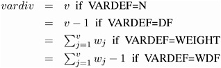
w j	weight for the j th variable from the WEIGHTS= option in the VAR statement. w j = 0 when either x j or y j is missing.
W	the sum of total weights. No matter if the observation is missing or not, its weight is added to this metric.
x	mean for observation x
y	mean for observation y
d ( x,y )	the distance or dissimilarity between observations x and y
s ( x,y )	the similarity between observations x and y

The factor is used to adjust some of the proximity measures for missing values.

Methods Accepting All Measurement Levels

GOWER	Gowers similarity
	To compute :	for nominal, ordinal, interval, or ratio variable,
			= 1
			for asymmetric nominal variable,
			= 1, if either x j or y j is present = 0, if both x j and y j are absent
	To compute :	for nominal or asymmetric nominal variable,
			= 1, if x j = y j = 0, if x j   y j ;
		for ordinal (where data are replaced by corresponding rank scores), interval, or ratio variable,
			= 1 ˆ’ x j ˆ’ y j
DGOWER	1 minus Gower
	d 2 ( x,y ) = 1 ˆ’ s 1 ( x,y )

Methods Accepting Ratio, Interval, and Ordinal Variables:

EUCLID	Euclidean distance
SQEUCLID	Squared Euclidean distance
SIZE	Size distance
SHAPE	Shape distance
	Note : squared shape distance plus squared size distance equals squared Euclidean distance.
COV	Covariance similarity coefficient
CORR	Correlation similarity coefficient
DCORR	Correlation transformed to Euclidean distance as sqrt(1-CORR)
SQCORR	Squared correlation
DSQCORR	Squared correlation transformed to squared Euclidean distance as (1-SQCORR)
L(p)	Minkowski ( L p ) distance, where p is a positive numeric value
CITYBLOCK	L 1
CHEBYCHEV	L ˆ
POWER( p, r )	Generalized Euclidean distance, where p is a non-negative numeric value, and r is a positive numeric value. The distance between two observations is the r th root of sum of the absolute differences to the p th power between the values for the observations

Methods Accepting Ratio Variables

SIMRATIO	Similarity ratio
DISRATIO	one minus similarity ratio
NONMETRIC	Lance-Williams nonmetric coefficient
CANBERRA	Canberra metric coefficient
COSINE	Cosine
DOT	Dot (inner) product
OVERLAP	Sum of the minimum values
DOVERLAP	The maximum of the sum of the x and the sum of y minus overlap
CHISQ	chi-squared
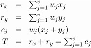
	If the data represent the frequency counts, chi-squared dissimilarity between two sets of frequencies can be computed. A 2 by v contingency table is illustrated to explain how the chi-squared dissimilarity is computed:
		Variable						Row sum
	Observation	Var 1	Var 2	...	Var v
	X	x 1	x 2	...	x v	r x
	Y	y 1	y 2	...	y v	r y
	Column sum	c 1	c 2	...	c v	T
	where
	The chi-squared measure is computed as follows :
	where for j = 1, 2, ..., v
	E ( x j )= r x c j /T
	E ( y j )= r y c j /T
CHI	Squared root of chi-squared
PHISQ	phi-squared
	This is the CHISQ dissimilarity normalized by the sum of weights
PHI	Squared root of phi-squared

Methods Accepting Symmetric Nominal Variables

The following notation is used for computing d ₂₈ ( x,y ) to s ₃₅ ( x,y ). Notice that only the non-missing pairs are discussed below; all the pairs with at least one missing value will be excluded from any of the computations in the following section because w _j = 0, if either x _j or y _j is missing.

M	non-missing matches
	, where
		= 1, if x j = y j = 0, otherwise
X	non-missing mismatches
		= 1, if x j   y j = 0, otherwise
N	total non-missing pairs
HAMMING	Hamming distance
	d 28 ( x , y ) = X
MATCH	Simple matching coefficient
	s 29 ( x , y ) = M/N
DMATCH	Simple matching coefficient transformed to Euclidean distance
DSQMATCH	Simple matching coefficient transformed to squared Euclidean distance d 31 ( x,y ) = 1 ˆ’ M/N = X/N
HAMANN	Hamann coefficient
	s 32 ( x , y ) = ( M “ X )/ N
RT	Roger and Tanimoto
	s 33 ( x , y ) = M /( M + 2 X )
SS1	Sokal and Sneath 1
	s 34 ( x , y ) = 2 M /(2 M + X )
SS3	Sokal and Sneath 3. The coefficient between an observations and itself is always indeterminate (missing) since there is no mismatch.
	s 35 ( x , y ) = M / X

The following notation is used for computing s ₃₆ ( x , y ) to d ₄₁ ( x , y ). Notice that only the non-missing pairs are discussed below; all the pairs with at least one missing value will be excluded from any of the computations in the following section because w _j = 0, if either x _j or y _j is missing.

Also, the observed non-missing data of an asymmetric binary variable can possibly have only two outcomes : presence or absence. Therefore, the notation, PX (present mismatches), always has a value of zero for an asymmetric binary variable.

The following methods distinguish between the presence and absence of attributes.

X	mismatches with at least one present
	, where
		= 1, if x j   y j and not both x j and y j are absent = 0, otherwise
PM	present matches
	, where
		= 1, if x j = y j and both x j and y j are present = 0, otherwise
PX	present mismatches
	, where
		= 1, if x j   y j and both x j and y j are present = 0, otherwise
PP	both present = PM + PX
P	at least one present = PM + X
PAX	present-absent mismatches
	, where
		= 1, if x j   y j and either x j is present and y j is absent or x j is absent and y j is present = 0 otherwise
N	total non-missing pairs

Methods Accepting Asymmetric Nominal and Ratio Variables

JACCARD	Jaccard similarity coefficient
	The JACCARD method is equivalent to the SIMRATIO method if there are only ratio variables; if there are both ratio and asymmetric nominal variables, the coefficient is computed as sum of the coefficient from the ratio variables (SIMRATIO) and the coefficient from the asymmetric nominal variables.
DJACCARD	Jaccard dissimilarity coefficient
	The DJACCARD method is equivalent to the DISRATIO method if there are only ratio variables; if there are both ratio and asymmetric nominal variables, the coefficient is computed as sum of the coefficient from the ratio variables(DISRATIO) and the coefficient from the asymmetric nominal variables.

Methods Accepting Asymmetric Nominal Variables

DICE	Dice coefficient or Czekanowski/Sorensen similarity coefficient
RR	Russell and Rao. This is the binary equivalent of the dot product coefficient.
BLWNM
BRAYCURTIS	Binary Lance and Williams, also known as Bray and Curtis coefficient
K1	Kulcynski 1. The coefficient between an observations and itself is always indeterminate (missing) since there is no mismatch.

Missing Values

Standardizing Variables

Missing values can be replaced by the location measure or by any specified constant (see the REPLACE option in the PROC DISTANCE statement and the MISSING= option in the VAR statement.) If standardization is not mandatory, you can also suppress standardization if you want only to replace missing values (see the REPONLY option in the PROC DISTANCE statement.)

If you specify the NOMISS option, PROC DISTANCE omits observations with any missing values in the analyzed variables from computation of the location and scale measures.

Distance Measures

If you specify the NOMISS option, PROC DISTANCE generates missing distance for observations with missing values. If the NOMISS option is not specified, the sum of total weights, no matter if an observation is missing or not, will be incorporated to the the computation of some of the proximity measures. See the Details section on page 1270 for formulas and descriptions.

Formatted versus Unformatted Values

PROC DISTANCE uses the formatted values from a character variable, if the variable has a format; for example, one assigned by a format statement. PROC DISTANCE uses the unformatted values from a numeric variable, even if it has a format.

Output Data Sets

OUT= Data Set

The DISTANCE procedure always produces an output data set, regardless of whether you specify the OUT= option in the PROC DISTANCE statement. PROC DISTANCE displays no output. Use PROC PRINT, PROC REPORT or some other SAS reporting tool to print the output data set.

The output data set contains the following variables:

• the ID variable, if any

• the BY variables, if any

• the COPY variables, if any

• the FREQ variable, if any

• the WEIGHT variable, if any

• the new distance variables, named from PREFIX= options along with the ID values, or from the default values.

OUTSDZ= Data Set

The output data set is a copy of the DATA= data set except that the analyzed variables have been standardized. Analyzed variables are those listed in the VAR statement.