2.13 Introduction to Audio Compression

The human auditory system (HAS) is complex and at various times works in the frequency domain to analyse timbre or in the time domain to localize sound sources. In practice the precision of the HAS is finite in both domains and if this precision is known, it is possible to render signals less precise than their original condition, but which still seem as precise to the ear. In practice few audio compression systems are used in his way. Instead lower bit rates are used and the coder attempts to minimize the audible damage.

There are a number of coding tools available, but none of these is appropriate for all circumstances. Consequently practical coders will use combinations of different tools, usually selecting the most appropriate for the type of input.

The simplest coding tool is companding: a digital parallel of the noise reducers used in analog tape recording. Figure 2.37(a) shows that in companding systems the input signal level is monitored . Whenever the input level falls below maximum, it is amplified at the coder. The gain that was applied at the coder is added to the data stream so that the decoder can apply an equal attenuation. The advantage of companding is that the signal is kept as far away from the noise floor as possible. In analog noise reduction this is used to maximize the SNR of a tape recorder, whereas in digital compression it is used to keep the signal level as far as possible above the distortion introduced by various coding steps.

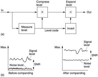
Figure 2.37: Digital companding. In (a) the encoder amplifies the input to maximum level and the decoder attenuates by the same amount. (b) In a companded system, the signal is kept as far as possible above the noise caused by shortening the sample word length.

One common way of obtaining coding gain is to shorten the word length of samples so that fewer bits need to be transmitted. Figure 2.37(b) shows that when this is done, the distortion will rise by 6 dB for every bit removed. This is because removing a bit halves the number of quantizing intervals which then must be twice as large, doubling the error amplitude.

Clearly if this step follows the compander of (a), the audibility of the distortion will be minimized. As an alternative to shortening the word length, the uniform quantized PCM signal can be converted to a non-uniform format. In non-uniform coding, shown at (c), the size of the quantizing step rises with the magnitude of the sample so that the distortion level is greater when higher levels exist.

In sub-band coding, the audio spectrum is split into many different frequency bands. Once this has been done, each band can be individually processed . In real audio signals many bands will contain lower-level signals than the loudest one. Individual companding of each band will be more effective than broadband companding. Sub- band coding also allows the level of distortion products to be raised selectively so that distortion is created only at frequencies where spectral masking will be effective.

Transform coding is an extreme case of sub-band coding in which the sub-bands have become so narrow that they can be described by one coefficient.

Prediction is a coding tool in which the coder attempts to predict or anticipate the value of a future parameter from those already known to both encoder and decoder. It can be used in the time domain or the frequency domain. When used in the time domain, a predictor attempts to predict the value of the next audio sample. When used in the frequency domain, the predictor attempts to predict the value of the next frequency coefficient from those already sent.

The prediction will be subtracted from the actual value to obtain the prediction error, also known as a residual, which is transmitted. The decoder also contains a predictor that runs from the same signal history as the predictor in the encoder and will thus make the same prediction. By adding the residual , the decoder's predictor will obtain the correct sample value. Provided the prediction error is transmitted intact, it will be clear that predictive coding is lossless.

In MPEG Layer 1 audio coding, the input is split into 32 bands and individually companded in each. A Layer 1 block is thus quite simple, containing 32 gain factors and 32 word length codes to allow deserialization of the 32 sets of variable length samples.

In MPEG Layer 2 coding, the same number of sub-bands is used, but further coding gain is possible because redundancy in the gain factors is explored allowing the same parameter to be used for several blocks.

In MPEG Layer 3 coding, a transform is performed that decomposes the spectrum into 192 or 576 coefficients, depending on the transient content of the signal. These coefficients are then subject to non-uniform quantizing followed by a lossless mathematical packing algorithm.

The MPEG AAC (advanced audio coding) algorithm represents an improvement over the earlier codecs as it uses prediction that can adaptively switch between time and frequency domain to give better quality for a given bit rate.