2.4 Blind Multiuser Detection: Subspace Methods
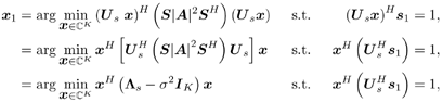
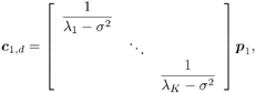
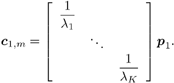
2.4 Blind Multiuser Detection: Subspace MethodsIn this section we discuss another approach to blind multiuser detection, which was first developed in [549] and is based on estimating the signal subspace spanned by the user signature waveforms. This approach leads to blind implementation of both the linear decorrelating detector and the linear MMSE detector. It also offers a number of advantages over the direct methods discussed in Section 2.3. Assume that the spreading waveforms Equation 2.72 where L s = diag ( l 1 , ..., l K ) contains the largest K eigenvalues of C r , U s = [ u 1 , ..., u K ] contains the K orthogonal eigenvectors corresponding to the largest K eigenvalues in L s ; and U n = [ u K + 1 , ..., u N ] contains the ( N - K ) orthogonal eigenvectors corresponding to the smallest eigenvalue s 2 of C r . It is easy to see that range ( S ) = range ( U s ). The column space of U s is called the signal subspace and its orthogonal complement, the noise subspace , is spanned by the columns of U n . We next derive expressions for the linear decorrelating detector and the linear MMSE detector in terms of the signal subspace parameters U s , L s , and s 2 . 2.4.1 Linear Decorrelating DetectorThe linear decorrelating detector given by (2.13) is characterized by the following results. Lemma 2.1: The linear decorrelating detector d 1 in (2.13) is the unique weight vector w Proof: Since rank ( U s ) = K , the vector w that satisfies the foregoing conditions exists and is unique. Moreover, these conditions have been verified in the proof of Proposition 1 in Section 2.2.2. Lemma 2.2: The decorrelating detector d 1 in (2.13) is the unique weight vector w Proof: Since Equation 2.73 it then follows that for w Proposition 2.3: The linear decorrelating detector d 1 in (2.13) is given in terms of the signal subspace parameters by Equation 2.74 with Equation 2.75 Proof: A vector w Equation 2.76 where the third equality follows from the fact that which in turn follows directly from (2.27) and (2.72). The optimization problem (2.76) can be solved by the method of Lagrange multipliers. Let Since the matrix L s - s 2 I K is positive definite, L ( x ) is a strictly convex function of x . Therefore, the unique global minimum of L ( x ) is achieved at x 1 , where Equation 2.77 Therefore, 2.4.2 Linear MMSE DetectorThe following result gives the subspace form of the linear MMSE detector, defined by (2.32). Proposition 2.4: The weight vector m 1 of the linear MMSE detector defined by (2.32) is given in terms of the signal subspace parameters by Equation 2.78 with Equation 2.79 Proof: From (2.34) the linear MMSE detector defined by (2.32) is given by Equation 2.80 By (2.72), Equation 2.81 Substituting (2.81) into (2.80) and using the fact that Since the decision rules (2.7) and (2.9) are invariant to a positive scaling, the two subspace linear multiuser detectors given by (2.74) and (2.78) can be interpreted as follows. First, the received signal r [ i ] is projected onto the signal subspace to get Equation 2.82 Equation 2.83 Therefore, the projection of the linear multiuser detectors in the signal subspace is obtained by projecting the spreading waveform of the desired user onto the signal subspace, followed by scaling the k th component of this projection by a factor of ( l k - s 2 ) -1 (for linear decorrelating detector) or Since the autocorrelation matrix C r , and therefore its eigencomponents, can be estimated from the received signals, from the discussion above we see that both the linear decorrelating detector and the linear MMSE detector can be estimated from the received signal with the prior knowledge of only the spreading waveform and the timing of the desired user (i.e., they both can be obtained blindly). We summarize the subspace blind multiuser detection algorithm as follows. Algorithm 2.5: [Subspace blind linear detector ”synchronous CDMA]
Equation 2.84 Equation 2.85 Equation 2.86 Equation 2.87
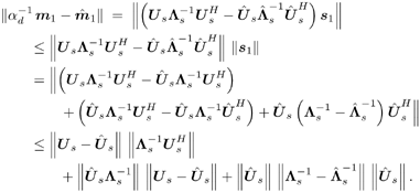
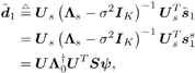
Equation 2.88 Equation 2.89 2.4.3 Asymptotics of Detector Estimates We next examine the consistency and asymptotic variance of the estimates of the two subspace linear detectors. Assuming that the received signal samples are independent and identically distributed (i.i.d.), then by the strong law of large numbers , the sample mean Equation 2.90 Equation 2.91 Similarly, First, for all eigenvalues and the K largest eigenvectors of Equation 2.92 Equation 2.93 Using the bounds above, we have Equation 2.94 Note that Equation 2.95 Equation 2.96 Therefore, we obtain the asymptotic estimation error for the linear MMSE detector, and similarly that for the decorrelating detector, given, respectively, by 2.4.4 Asymptotic Multiuser Efficiency under Mismatch We now consider the effect of spreading waveform mismatch on the performance of subspace linear multiuser detectors. Let Equation 2.97 with Equation 2.98 Equation 2.99 For simplicity, in the following we consider the real-valued signal model [i.e., A k > 0, k = 1, ..., K , and n [ i ] ~ N ( , s 2 I N )]. [Here N ( ·, ·) denotes a real-valued Gaussian distribution.] The signal subspace component Equation 2.100 for some
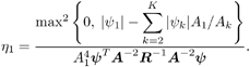
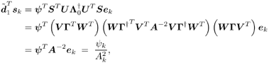
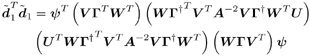
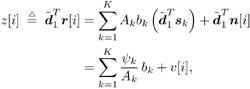
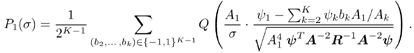
Equation 2.101 which measures the exponential decay rate of the error probability as the background noise approaches zero relative to that of a single-user system having the same signal-to-noise ratio. A related performance measure, the near “far resistance , is the infimum of AME as the interferers' energies are allowed to vary arbitrarily. Equation 2.102 Since as s Equation 2.103 Next we compute the AME and the near “far resistance of the two subspace linear detectors under spreading waveform mismatch. Define the N x N diagonal matrices Equation 2.104 Equation 2.105 Denote the singular value decomposition (SVD) of S by Equation 2.106 where the N x K matrix G = [ g ij ] has g ij = 0 for all i Lemma 2.3: Let the eigendecomposition of C r be C r = U L U T . Then the N x N diagonal matrix Equation 2.107 where G Using the result above, we obtain the AME of the subspace linear detectors under spreading waveform mismatch, as follows. Proposition 2.5: The AME of the subspace linear decorrelating detector given by (2.74) and that of the subspace linear MMSE detector given by (2.78) under spreading waveform mismatch is given by Equation 2.108 Proof: Since d 1 and m 1 have the same AME, we need only to compute the AME for d 1 . Because a positive scaling on the detector does not affect its AME, we consider the AME of the following scaled version of d 1 under the signature waveform mismatch: Equation 2.109 where the second equality follows from the fact that the noise subspace component Equation 2.110 Equation 2.111 Equation 2.112 The output of the detector Equation 2.113 where Equation 2.114 It then follows that the AME is given by (2.108). It is seen from (2.114) that spreading waveform mismatch causes MAI leakage at the detector output. Strong interferers ( A k >> A 1 ) are suppressed at the output, whereas weak interferers ( A k << A 1 ) may lead to performance degradation. If the mismatch is not significant, with power control, so that the open -eye condition is satisfied (i.e., |
 range (
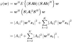

 0, the two linear detectors become identical, as we would expect.
 j
j  g 22
g 22 
EAN: 2147483647
Pages: 91