11.3 Spectral Balancing (Iterative Water-Filling)
11.3 Spectral Balancing (Iterative Water-Filling )Spectral balancing can be defined as a wide class of methods where systems may alter their power spectral densities for the common good of all DSL systems. This may be performed autonomously, and can be used with or without coordination. Generally, autonomous DSM improves all DSL systems' performance with respect to their current performance level (even if some have a fixed, nondynamic spectra). The more systems that execute DSM, the larger the improvements for all. The situation for spectral balancing refers to the "interference channel" in information theory that appeared earlier in Figure 11.9. Each DSL transmitter and receiver are of the usual type for the line, but the spectra used may be varied dynamically in response to the crosstalking situation in the binder. The interference channel best spectra and rate regions remains an unsolved problem in information theory today. However, Section 11.3.1 introduces a very good method known as iterative water-filling, developed by Yu and Rhee [24] and investigated for DSL/DSM by Yu. Iterative water-filling may often be close to optimum, can be used to generate rate regions, and leads to enormous performance improvements with respect to existing practice of SSM in DSL. It also admits a distributed implementation with no need for coordination (which may not be admitted by absolutely optimum solutions whenever they are found). Lastly, a solution found by iterative water-filling will do no worse than those chosen by existing standards in static SM, so there is never any degradation with respect to existing practice. Section 11.3.2 then proceeds with examples of the large improvements possible using iterative water-filling. 11.3.1 Yu's Iterative Water-fillingWater-filling is an algorithm well known in DSL because most DMT-based modems use it (or approximations to it) to decide the energy and information distribution for the modem adaptively as a function of line conditions. Wei Yu, assisted by colleague G. Ginis, noticed that a certain optimization procedure used in multiple-access spectrum optimization that he was studying has an interpretation of being equivalent to several iterative and successive uses of the water-filling procedure that is optimum for a single- user channel. Water-filling is illustrated for a single point-to-point channel in [1]. The spectrum is found by plotting the inverse of the SNR(f) for the channel and filling that inverse curve with water/power until all power available has been used. The water power will lay at a constant level as shown in Figure 11.16. Mathematically, the sum of the noise-to-signal ratio at each frequency plus the power spectral density at that same frequency must equal a constant (the water level): Figure 11.16. Iterative water-filling concept. where f can represent a discrete set of tones in a DMT system, The highest spectral efficiency achievable at each tone or spectral point is computed as and practical systems usually use a code with some constant gap to capacity (including any needed margin) and so follow a similar equation where b n is the number of bits transmitted in the n th subchannel's QAM symbol, and the data rate for a single user is thus A set of U = L users, each with data rate R l on the line (combined perhaps into a vector of data rates R = [ R 1 R 2 ... R L ]), has an average rate provided by [3]
for which an objective might be maximization, and is equivalent to maximizing the sum of the data rates of the lines. In general, one user's line rate might be more important than that of another and so a weighting could be assigned to each channel m l such that which will equal Iterative water-filling can be optimum in some cases and leverages the observation that if all spectra except one users' spectrum are held constant, then the resulting solution is again a water-fill solution with other users channel-filtered energy at any frequency being viewed as a component of the noise spectra at that frequency. Clearly then, a necessary (but not always sufficient) condition for an optimum solution would be that each and every user's spectra individually satisfied a water-filling constraint with the sum contributions of the other water-filling spectra included. Both Chung [37] and Leshem [38] have shown that such a point, often called a "Nash equilibrium," always exists. Chung [39] has also shown that the IW procedure will converge to it for DSL. For the simple rate-sum maximization, the iterative water-filling process is simple ”just cycle through water-filling problems for all users (starting initially with one user and all others zeroed or perhaps initialized to using flat spectra) several times. The process will converge to a solution that satisfies the water-filling condition simultaneously for all users necessarily . This procedure applies directly when all the users have equal rate, so that the average rate (or sum rate) is desired to be as large as possible. A method to approximating, but lower bounding, the rate region for the interference channel was also provided by Yu. The iterative water-filling procedure in Figure 11.16 could be augmented by an outer set of loops for each of the users that would reduce the transmit power constraint individually for one of the users for each execution of iterative water-filling. Each user will individually lower power, then transmit the necessarily lower (or the same) data rate, while other users may see an increase. Running through possibilities of reduced power on all users in all combinations over some grid of possible power sets should also trace a region of implementable and achievable rates for spectral balancing on the interference channel. This region lower bounds the rate region. It is the rate-region achievable with iterative water-filling. Distributed Water-fillingYu's power loop suggests a mechanism for avoiding essentially all coordination in spectrum balancing. If each DSL system independently executes water-filling at a presumably slow speed of spectrum change, the entire system implements iterative water-filling in a distributed fashion, assuring the maximum sum of total data rates for the given power levels. Thus, no coordination is necessary. Today, ADSL modems are a good example of an interative water-filling system, except that they often rate-adapt, or worse yet, margin-adapt instead of minimizing transmitted power. However, they are well known to always converge in the RA, MA, or FM mode of operation. A DSL system having excessive margin, or equivalently, a higher data rate, should have its power decreased (which can be done automatically by that system until margin at the desired data rate is the minimum acceptable). This is a FM (fixed margin) operation when the power is minimized at a fixed margin sufficient to ensure excellent performance. The use of FM mode improves other systems that otherwise would have insufficient margin. Coordination is unnecessary as long as the attempted data-rate-tuple is in the achievable rate region of iterative water-filling. Coordination in the form of the SMC knowing the rate region more accurately allows a DSM-coordinated iterative water-filling system to more aggressively chose points near the boundary of the achievable rate region. Clearly, just a small amount of coordination in terms of knowing which systems have excessive margin, and permitting or not permitting them to exploit it based on other system's margins and data rates, allows further distributed water-filling improvement. Discussions with several service providers reveal that their SMCs do indeed already store data rate (and line length also) for all DSL lines. 11.3.2 Examples of ImprovementsThis section provides four examples of the benefit of iterative water-filling: (1) RT-located-ADSL FEXT into co-located ADSL; (2) 10MDSL to/from ADSL (and VDSL), (3) ADSL to/from VDSL; and (4) mixture of asymmetric and symmetric VDSL service in the same binder. RT-Located-ADSL FEXT into CO-located ADSLFigure 11.17 comes from [29] and illustrates a basic problem in ADSL deployment that is solved by iterative water-filling in DMT ADSL modems (when the FM mode option is selected). Several authors and at least four companies have independently verified the improvements in [28], [30], [31], [32]. Figure 11.17. Illustration of RT-located-ADSL FEXT into CO-located ADSL (for Verizon experiment in [31], no line 3, and line 1 is 20 kft, while line 2 is 14 kft fiber, 6 kft copper ). The ADSL receiver on line 1 in Figure 11.17 will sense large FEXT from the RT-located ADSL downstream transmitters on lines 2 and 3, both of which are only 5 kft away from the ADSL receiver. Under nominal static spectrum management (T1.417,[5]) assumptions, line 1 has very low data rate ”that is, the achievable data rate is 300 kbps downstream. Verizon [31] reports this problem also for the case where line 1 is 20,000 feet long, and the RT on line 2 (there is no line 3 in Verizon results) is 6000 feet from the line 1 receiver (or 14,000 fiber feet from central office). In the Verizon case, the line 1 data rate is only 100 kbps, whereas line 2 happily trained to over 9 Mbps. Both were operated in rate-adaptive (RA) mode. Clearly, line 2 is "hogging" line 1's possible data rate with strong FEXT. Instead, if both lines 1 and 2 are operated with FM training, so the iterative waterfilling now works to minimize power at 6 dB of margin, and the rate region in Figure 11.18 is obtained. A good operating point might be to hold the short line (2) to 2 Mbps, in which case the long line (1) gets nearly 1.8 Mbps also ” a factor of nearly 20 increase in data rate on the long line. Table 11.1 illustrates the improvements/choices for the Verizon experiment. Note the sum of data rates is highest in RA mode, but line 1 does not get much data rate as line 2 takes all. Figure 11.18. Fixed-margin iterative water-filling achievable rate region for Verizon experiment in [31]. Telcordia [32], Voyan [28], and Stanford [30] all report also on the situation exactly shown in Figure 11.17 with line 3 present and absent. The long line 1 data rate is limited to 300 kbps again because of ADSL FEXT. Figure 11.19 illustrates the rate regions in this case for lines 1 and 2 with line 3 silent. Clearly, the data rate of line 1 can be improved by a factor of nearly 10, to almost 3 Mbps. Figure 11.19. Rate regions for lines 1 and 2 with line 3 off (top); for lines 1 and 3 with 2 held at 1.6 Mbps (bottom). The rate region on the right in Figure 11.19 shows the data rates when line 2 is held at 1.6 Mbps ”clearly here, 1.5 Mbps is possible on each of the other two long lines. This represents a factor of 4 increase in data rate with respect to the case where line 2 can "hog" the capacity of the binder. Absolutely no coordination is used in Figures 11.18 or 11.19. The operator simply sets the data rate of the short-line modem less aggressively and operates all modems in FM mode. The question of spectra is also of interest corresponding to the rate region points. For instance, in the case of the right-hand plot in Figure 11.19, the spectra were nearly flat and had the following levels:
Note that line 2 did not turn off at low frequencies, so this is not in this case an FDM-like solution, but rather simply reduced its transmit spectrum by a large amount. In more extreme cases, like the Verizon experiment of Figure 11.18 and [31], the line 1 spectra was concentrated at low frequencies 35 “100 at high power-spectral-density level, whereas line 2 was above tone 100 at a very low power-spectral-density level. In each case, the spectra will adapt to the correct point in the rate region with the corresponding spectra, no matter which line starts first. 6 dB of fixed margin was used in all plots. Table 11.1. Illustration of Gains on Long Line for Verizon Expt.
In practice, the FM operation has such a wide range of signals, it is implemented in two parts :
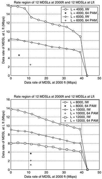
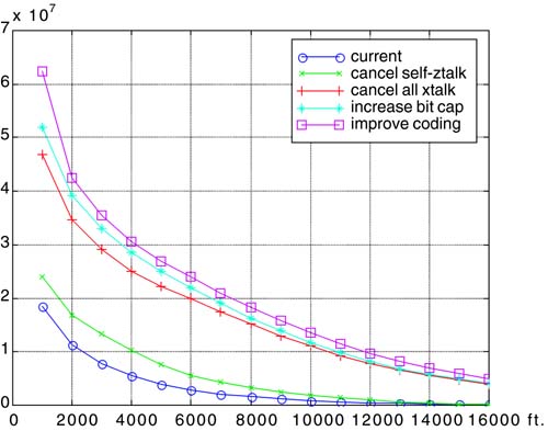
The initial politeness back-off allows conversion devices (e.g., ADCs and DACs) to be operated with full precision when large amounts of power reduction are present on short lines. Doing the entire back-off with swapping could lead to precision loss in the converters, so politeness is used to avoid this implementation problem. 10MDSL, self, and into ADSL and VDSL10MDSL is, at the time of this writing, a new standards project in the United States. The objective is basically 10 Mbps symmetric transmission on 1 or more DSL lines. Clearly with static SM, the upstream transmission of 10 Mbps creates a strong crosstalking NEXT into downstream ADSL (or VDSL). Basically ”without the iterative water-filling DMT method in FM mode illustrated here ”this 10MDSL is not feasible technically as the upstream from static spectra will annihilate downstream ADSL. To solve the problem, both directions of transmission in a DMT modem (this time using up to 1024 tones) are allowed to adapt in FM mode, thus determining NEXT and FEXT on a per-binder best basis for the selected data rates of all the DSL modems. The first concern will be 10MDSL upstream into 10MDSL downstream, and then the combinations with ADSL and VDSL will be illustrated. Figure 11.20 illustrates that static-spectra such as a 64 PAM ("SH"DSL) modem has very poor range on a single line, slightly more than 2000 feet. This number has been verified by a number of groups [33] who report from 2000 feet to 2500 feet, depending on noise and coding-gain assumptions. For the same coding gain of 3.8 dB, the FM-mode DMT system achieves 5000 feet (or equivalently gets 4x the data rate at 2000 feet). Voyan has verified the 5000-foot range point in [34]. Figure 11.21 shows the more realistic situation of mixture of various loop lengths of 10MDSL, and instead now plots rate regions. Figure 11.21 holds 1/2 the lines (12 MDSLs) at 2000 feet and varies the length of the another 12 between 2000 feet and 12,000 feet to see the achievable rates. Again the FM-mode interative water-filling maintains the 5000 foot range of 10 Mbps, but also allows very high data rates on the short loop while the long loops are doing quite well. Table 11.2 summarizes the goals of the 10 MDSL project, along with what was achieved in the FM mode, which leaves a considerable margin for error with respected to the project goals. Figure 11.20. 10Mbps symmetric DSL (10MDSL) on a single-line with 25 lines all of same length. No coordination used. Figure 11.21. Illustration of self-10 MDSL rate regions with with DSM's iterative water-filling. Table 11.2. Augmentation of 10 MDSL results with FM-IW (DMT) Results
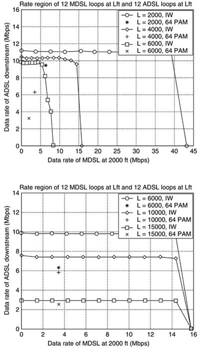
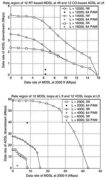
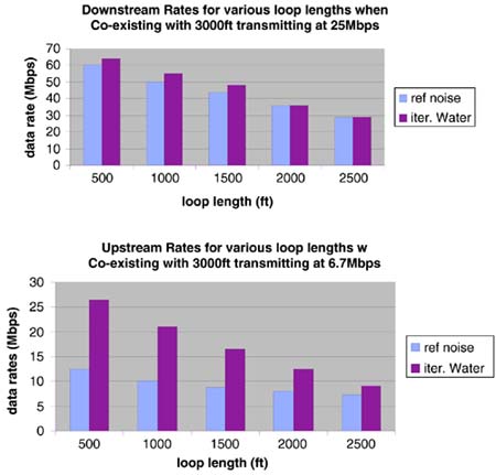
Figure 11.22 also provides some rate regions for ADSL with 10 MDSL. When deployed from the same point, the rate regions are very rectangular, indicating little effect (because of the iterative water-filling) of 10 MDSL on ADSL range. Figure 11.23 illustrates the interesting and highly likely possibility of an existing CO-deployed ADSL in a binder with a new 10 MDSL at an RT ”the situation of Figure 11.17 is repeated with the 10MDSL on line 2, which is 4000 feet beyond the fiber terminal at 10,000 feet and various lengths of line 1. Figure 11.22. Illustration of rate regions of 10 MDSL with ADSL (deployed from same point). Figure 11.23. Illustration of remote-10 MDSL (10 kft from CO) and ADSL located at CO, and also MDSL/VDSL rate regions (bottom). Figure 11.23 clearly illustrates the annihilation of the ADSL circuit with static spectra “like SHDSL systems, while the DSM-based iterative water-filling is showing some degradation to ADSL, but data rates of 1.5 “2 Mbps are preserved even in the presence of 10 MDSL. Clearly, static spectra (in this case particularly SHDSL PAM solutions) fail horribly, while the DSM provides a very clear advantage that is overwhelming. Figure 11.23 on the bottom illustrates the VDSL and 10MDSL rate regions. Again, static spectra (see the points on left in Figure 11.23 close to horizontal axis) are failing to meet requirements while DSM is clearly functioning at very high rates. For more information, see [30]. ADSL to/from VDSL ExamplesA problem feared by service providers in potential deployment of VDSL is the downstream FEXT that VDSL ONU emits into the ADSL downstream receivers attached to lines in the same binder. For instance, the situation investigated in Figure 11.24 has a VDSL ONU at 3000 feet from its customer, and ADSL central office at 9000 feet from its customer. Both customers are at approximately the same location. VDSL downstream signals below 1.1 MHz create a large FEXT for ADSL, severely reducing its performance under static spectrum management. Some studies leading to [28] have found the interaction to be so detrimental to the performance of both ADSL and VDSL, leaving static SM with a difficult trade-off that discouraged VDSL deployment. Figure 11.24. Rate region for ADSL and VDSL example. Iterative water-filling again solves the interference problem, providing good rates for both ADSL and VDSL beyond requirements. Under this new presumption of both modems converging to the iterative water-filling solution creates the rate region of Figure 11.24. Figure 11.24 illustrates downstream rate region for 4 VDSL modems at 3000 feet and 4 ADSL modem at 9000 feet (both on 26 gauge). All four ADSL modems have the same spectrum and so do all four VDSL modems in this case because the line lengths and impairments are the same (it would be hard to draw the 8-dimensional region, but we also wanted to ensure more than just one crosstalker for each of ADSL and VDSL as that would lead to data rates larger than those in Figure 11.24). The upstream data rates are not shown, but are 3 Mbps for VDSL and 500 kbps for ADSL. The nominal situation of T1.417, using the 998-standardized spectrum for VDSL of “60 dBm/Hz, causes the downstream rate for ADSL to be the 1.5 Mbps best case, while VDSL hopes to achieve 18 Mbps downstream in recent standards. Clearly, the rate regions here indicate that the VDSL systems can operate at 25 “26 Mbps, while the ADSL system operates somewhere between 4 and 5 Mbps. The spectra of the two signals is shown in Figures 11.25 “11.27 for various power levels of the ADSL and VDSL. Note that the ADSL signals tend to operate a full power, but over very different bandwidths as the iterative water-filling determines a cut-off frequency that is a function of the data rate attempted on the ADSL line. The VDSL signal does not vary so much in used band , but does vary power level automatically with margin-adaptive water-filling used (which can be implemented to implement the lowest power to achieve a given margin of 6 dB at a given data rate as in our examples). The VDSL PSD level varies over a wide range, taking only as much power as is necessary to implement a target bit rate (say 26.6 Mbps) while then reducing crosstalk into the ADSL so its performance then increases . Figure 11.25. ADSL and VDSL spectra when at full power (2.48 Mbps, 26.6 Mbps). Figure 11.27. ADSL and VDSL spectra at intermediate condition [3.1, 26.6 ] Mbps. Figure 11.26. ADSL and VDSL spectra with full ADSL power, but low VDSL power (7.19, 16.2) Mbps. Figures 11.28(a) and (b) show the rate regions as the length of the VDSL or ADSL lines are varied, respectively. Figure 11.28(a). VDSL/ADSL with varying VDSL line length. Figure 11.28(b). VDSL/ADSL with varying ADSL line length. VDSL ExamplesAs an alternative, this subsection investigates some trade-offs in VDSL when iterative water-filling is used for a 1000-foot loop and a 3000-foot loop. Our investigations in this section are actually done for 4 loops at 3000 feet and 4 loops at 1000 feet. The objective here is to determine what symmetric services might be offered on the 1000-foot loops while the 3000-foot loops maintain a 26/3 Mbps asymmetric VDSL service. Any point in the upstream rate region in Figures 11.29 and 11.30 can be paired with any point in the downstream rate region of Figures 11.29 and 11.30. In 1999, various service providers argued as to the relative merits of asymmetric versus symmetric service, eventually reaching a compromise where no group saw a data rate it liked with 18 Mbps/1.5 Mbps downstream service being argued by one group of service providers as perhaps the bare minimum for video service, whereas 6 Mbps symmetric was argued by another group to be below what they wanted but perhaps interesting. Figure 11.29 shows that even within the 998 plan of VDSL, DMT water-filling VDSL modems avoid each other within the common band in a mutually beneficial way autonomously, leading to 26/6 Mbps on a worst-case 3000-foot VDSL loop and at least 20 Mbps symmetric on the 1000-ft loop. Such a situation might well occur in practice with residential loops being further than small business loops. In any case, the data rates significantly exceed those that were projected by static spectrum management. Figure 11.36 alters the cut-off frequencies of up and down, given that with DSM, the 998 plan may not have provided the best trade-off. Indeed, that leads to 26/13 Mbps on the asymmetric VDSL loop at 3000 ft while the 1000 ft loop has at least 30 Mbps symmetric service. These cut-off frequencies for up/down need not be fixed if DSM is used. Figure 11.29. VDSL 998 upstream and downstream rate regions for 4 each of 1000 and 3000 ft loops in same binder with distributed Level 0 iterative water-filling. Figure 11.30. VDSL flexible upstream and downstream rate regions for 4 each of 1000 and 3000 ft loops in same binder with Level 0 distributed water-filling, but Level 1 control of up/down cut-off frequencies. Figure 11.36. Vectored ADSL data rates versus range. Figure 11.31 illustrates the trade-off versus line length as the loop length of VDSL instead varies with respect to the best-known (and not used because it cannot be implemented in the static-spectra-only QAM VDSL) reference-noise, spectrally shaped, power back-off methods of VDSL and the corresponding ADSL data rates. Figure 11.31. Downstream data rate comparisons with 4 lines at 3000' at 25 Mbps; Upstream data rate comparisons with 4 lines at 3000' at 6.7 Mbps. |
| Top |
EAN: 2147483647
Pages: 154
- The Effects of an Enterprise Resource Planning System (ERP) Implementation on Job Characteristics – A Study using the Hackman and Oldham Job Characteristics Model
- Context Management of ERP Processes in Virtual Communities
- Intrinsic and Contextual Data Quality: The Effect of Media and Personal Involvement
- A Hybrid Clustering Technique to Improve Patient Data Quality
- Development of Interactive Web Sites to Enhance Police/Community Relations