INTERPRETING CAPABILITY RESULTS

For a short- term capability study, if the ±4 limits are both within specification, the machine is considered capable. In other words, we have determined that the machine has sufficient capability to allow for process shifts (different materials, operators, tool wear, etc.) and yet still maintain an overall long-term process output of 99.73% within specification. When this is the case, the capability analysis sheet will appear as in Figure 12.15.

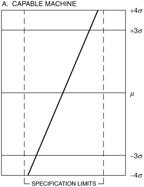
Figure 12.15: A machine capable within a ±4 sigma.

Typically, if the machine is not capable, one of two symptoms (or both) may be present and show up in the graph as in Figure 12.16.

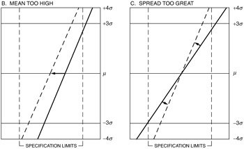
Figure 12.16: A machine that is not capable.

How would each of these problems be solved ? Note that the capability analysis sheet provides a different "view" of the process distribution. The four illustrations in Figure 12.17 reflect the relationship between the process capability analysis sheet and the specifications on the process distribution.

 
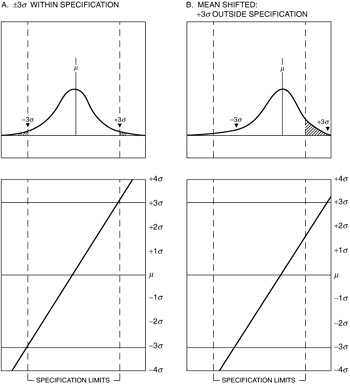
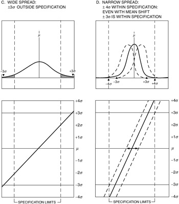
Figure 12.17: Process capability and specifications.

Let us return at this point to our capability analysis sheet for the Shaft O.D. Appropriate questions are: Is the process capable? Why? Why not? If the process is not capable, mark the reasons why on your capability analysis sheet. If the process is not capable, what will have to be done to make it capable?

Note that in a case of this kind, or any other process that has been shown to be not capable, it would be necessary to determine the causes of variation; especially if the casual factor noted included the spread of the process. Table 12.1 provides a number of causes that originate from various process elements that might in turn yield noncapable output.

Table 12.1: A Number of Causes That May Contribute to a Noncapable Process

Elements of the Process	Typical Variable Characteristics
People	Accuracy of adjustment, cleanliness, fatigue, expertise, experience, tool setup, choice of speeds, part feed
Maintenance	Lubrication, longer-term adjustment and calibrations, replacement of worn parts , setup, tooling, age/design, maintenance
Environment	Ambient temperature, humidity, dust, constancy of power supply ” electrical, pneumatic, etc. ” contamination
Materials	Uniformity, hardness, dimensions, cleanliness
Methods and procedures	Rate of production, pattern of assembly, layout inspections
Machines	Backlash or clearance of gears or bearings, accuracy of adjusting devices, speed consistency, sensitivity to operating temperature, rates of component wear
Tools	Dimensional accuracy, wear

Our discussion would not be complete without addressing the issue of setup verification. First, we define setup verification as an established number of consecutive gaged samples (minimum of three, unless specifically covered by an individual department procedure) used to target a process before, and sometimes during, an operation or production run. This setup sample data collection is independent and is in addition to the regular control plan charting requirements.

Second, now that we have defined it, let us examine when setup verification may be required. Setup verification is required after at least the following occurrences:

• Significant machine repair

• Tool change

• Replacement or repair of tool holders

• Repair of part chucks, locators, collets, expanders, or fixtures

• Replacement of polishing shoes, paper, or burnishing rollers

• Punch or die changes

Finally, setup verification is considered complete when the plot point is within the setup target zone. At that point, the regular required control plan frequency checks are performed.

If the point is not within the setup target zone, make adjustments and repeat the verification check. If unable to reach the setup verification target, notify the supervisor and appropriate maintenance personnel. At this stage of verification, control charts should have a target setup arrow and target zone identified.

An alternative graphical evaluation method may be to use graph paper (see Figure 12.18). The difference is that using graph paper allows the data to be collected on the left bottom of the graph, with the histogram right above it in the form of a check sheet, and then moving to the right, there are columns already identified for the count ( f ) of each cell , the cumulative sum of the counts ( f _i ), and the cumulative percentage ( f _i %). To the right is the probability graph paper, where the plotting is done as before. In this form of graph, however, the analyst can get a rough idea about the average as well as about the rejects on both extremes of the population if they do go outside the specification limits. All of the information is on the same page.

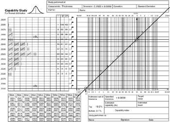
Figure 12.18: Histogram and probability combination form.

In the case of nonnormal distribution there is a log-log paper that can transform the data into normal distribution, and then the process of evaluating is exactly as that for the normal plotting. Figures 12.19 and 12.20 show what can happen when nonnormal data are plotted on the probability paper and what should happen when the data are plotted on the appropriate graph.

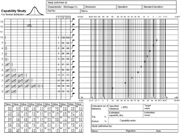
Figure 12.19: Nonnormal data plotted on normal probability paper.

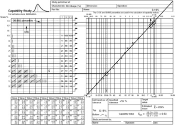
Figure 12.20: Nonnormal data plotted on log log graph.

For the nonnormal transformation, the following formulas must be used to calculate graphically the C _p and C _pk :

C _p = total specified tolerance · 99.99865 percentile - 0.135 percentile