CAPABILITY INDICES | Six Sigma and Beyond: Statistical Process Control, Volume IV

Earlier we made the distinction between short- and long- term capability. In this section, we will define the terms and show the actual calculations for each. Table 12.2 identifies the capabilities and puts them in relation to each other.

Table 12.2: Capability Indices
Preliminary	Ongoing	Potential (measures precision only)	Capability (measures precision and location)
P _p Process potential	C _p Process potential	P _p	P _pk
P _pk Process capability	C _pk Process capability	C _p	C _pk

To differentiate between the two capabilities think of preliminary process capability as a short-term assessment of process performance relative to customer requirements. In other words, with preliminary process capability, we obtain early information on new or revised processes. On the other hand, ongoing process capability is a long-term assessment of process performance or output and its ability to meet specifications.

Another way of separating the two concepts is to think in terms of what we want and what we get. The first has to do with our expectations of the preliminary capability; the second has to do with the actual, ongoing delivery of what we want.

To calculate preliminary process capability, we need the process to be in control and stable. (To accomplish this, we define the short-term capability in such a way that all the known assignable causes, such as setup, tooling, and material, are removed from the data. However, we compensate for this in our expectation of the capability index.) Second, we need to know

Specification limits (including nominal value)
Mean of process output population, ¼ _x
Standard deviation of process output population, ƒ _x
Shape of process output distribution (Because of our assumption, in most cases, this turns out to be a normal distribution.)

Preliminary process capability makes sense only if there is a stable process; otherwise , the capability is worthless. Some guidelines for improvement include:

If P _p > 1.67 and P _pk < 1.67, move process mean closer to target.
If P _pk ‰ 1.67, process is normally acceptable for production.
If P _pk ‰ 1.67, then the process is not normally ready for production.
Always pursue higher P _pk in the name of continual improvement.
The higher the P _p and the P _pk , the more desirable the capability.

To calculate ongoing process capability, we need the process to be in control. In addition, we need to know the following:

Specification limits (including nominal value)
Mean of process output population, ¼ _x
Standard deviation of process output population, ƒ _x
Shape of process output distribution

Process capability makes sense if and only if there is a stable process; otherwise, the capability is worthless. The following are some guidelines about improvement:

If C _p < 1.33, then improve performance.
If C _p > 1.33 and C _pk < 1.33, then move closer to target.
Always pursue higher C _pk in the name of continual improvement.
The higher the C _p and the C _pk , the more desirable the capability.

A 3-sigma process has a C _pk of 1, a 4-sigma process has a C _pk of 1.33, and a 6-sigma process has a C _pk of 2.00. If the mean is on target, then Ppk = C _pk means that the process is centered. In general, the distance from the process mean to the nearest specification limit in a k-sigma process is k ƒ .

To ensure that the reader understands the concept of P _pk and C _pk , let us try an analogy with the basketball hoop and the basketball itself. The hoop is designed to accommodate only one regulation basketball, for scoring purposes. The hoop will not change, and it will always accommodate one ball at the time. Its potential is fixed. However, if basketball is played with different sizes of balls, the potential increases or decreases depending on the size of the ball. For example, it is impossible to throw a beach ball through the hoop, no matter what. On the other hand, there are many golf balls or baseballs that may fit through the hoop at the same time. In the first case, the capability is very small (in fact, impossible ), and in the second, the capability is large. In both cases, the index tells us the limitation of the capability and the relation to the specifications.

Another advantage of knowing the C _p and C _pk is that once these values are known, one can determine the shape of the distribution. Similarly, once we know the shape of the distribution, the mean, and the specifications, we can calculate the C _p or C _pk . For example, in Figure 12.21, we are given that the distance from the target value to the LSL is 12 units, and the distance from the mean to -3 sigma is 9 units. To calculate the C _p and C _pk , we do the following:

C _p = total specified distance/6 = 24/18 = 1.33. (If half the distance is 12 units, the total is 24. The distance of -3 sigma to the mean is 9 units; therefore the difference for the entire 6 sigma is 18 units.)
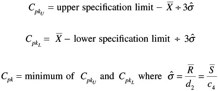
C _pk = min of C _pkU and C _pkL where = Rbar/d ₂ = Sbar/c ₄ .
C _pkU = USL-Xbar/3 = 12/9 = 1.33 (We know from the picture that the distance from the mean to the USL is the same as the distance from the LSL to the mean, which is equal to 12. Therefore, the entire distance is 24. The target is half of the total specification (24/2 = 12). The 3 is given as 9 units.)
C _pkL = Xbar - LSL/3 = 12/9 = 1.33 (We know from the picture that the target is half of the total specification [24/2 = 12]). We are given the distance from the target to the LSL, which is equal to 12 units. The 3 is given as 9 units.)

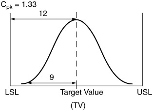
Figure 12.21: C _pk example.

So, in this case, the C _pkU = C _pkL = 1.33. Therefore the C _pk is 1.33. The fact that they are the same also indicates that the distribution is centered. The centerness is also supported by the fact that the C _p is also 1.33.

A second example will demonstrate the C _p and C _pk relationship (see Figure 12.22).

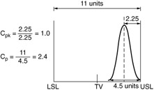
Figure 12.22: C _p and C _pk comparison example.

We will use the same rationale and formulas that we used in the last example. So, we are given the distance of the mean of the distribution to the USL as equal to 2.25 units; this is also the 3 distance (4.5/2 = 2.25). The 6 for the distribution is given as 4.5 units. The Xdouble bar = 3.25 (11 total units/2 = 5.5 units for the target; 5.5 - 2.25 = 3.25 the center of the distribution. = .75 [3 = 2.25, so = 2.25/3]). Now we can calculate the capability indices as follows :

C _p = Total specified distance/6 = 5.5 - (-5.5)/6(0.75) = 11/4.5 = 2.4

C _pk = min of C _pkU and C _pkL where = Rbar/d ₂ = Sbar/c ₄

C _pkU = USL - Xbar/3 = 5.5 - 3.25/3(0.75) = 2.25/2.25 = 1.0

C _pkL = Xbar - LSL/3 = 3.25 - (-5.5)/3(0.75) = 8.75/2.25 = 3.89

Therefore, C _pk = 1.0 because this is the minimum value of the two. What does this mean? The C _p tells us that there is room (in fact, approximately 2.5 times) to move about the specifications. There is a potential capability in here that is not being utilized. The C _pkU tells us that we are so close to the USL that even the smallest deviation, a "wiggle," in our process will create nonconforming items. The C _pkL , on the other hand, tells us that there is more than sufficient capability on the lower end of the distribution, and given this process, chances are that we will not have nonconforming items on the low end.

So, what should be the decision? In this case, because the distribution seems to be in good shape and the variation is very tight; we should adjust the target of the distribution toward the target of the specification. In this case, rather than aiming the target to 3.25 units, we should move it closer to the 5.5 units.

A third example will demonstrate the reverse. That is, knowing the capability indices and specifications, we can actually figure out what the distribution looks like. This is shown in Figure 12.23. In Figure 12.23a, the information is given, and in Figure 12.23b the distribution is shown.

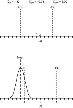
Figure 12.23: Information for drawing the distribution shape from capability indices and specifications.

In Figure 12.23a, we already know what the total specification is (8 units); we also know the target (8/2 = 4); and of course, we are given the indices. Because we know that the indices are different, we know that the distribution is not centered. In fact, we already know that at the lower end of the specifications, we should expect nonconformances. We know this by the C _pkL , which is -0.33. We can proceed, then, with the calculations.

. At this point we know that the spread for the ±3 sigma is equal to six units (6 = 6).
C _pkU = USL - Xbar/3 ; 3.00 = USL - Xbar/3; USL - Xbar = 9. This is the distance from the mean to the USL. So, in our example, we count nine units to the left from the USL, and that point is the center of our distribution. Numerically, this point is -5. (we can also calculate this by substituting into the equation [4 - Xbar = 9]; Xbar = -5)
C _pkL = Xbar - LSL/3 ; -0.33 = LSL - Xbar/3; LSL - Xbar = -1. This is the distance from the mean to the LSL. Numerically, this point is -4. (we can also calculate this from substituting into the equation [LSL- (-5) = -1]; LSL = -1).

Now that we know what the mean (-5) and the spread of the distribution (six units) are, we can draw the curve as in Figure 12.23b. As we suspected, the lower end of our distribution will have nonconformities . However, because the variation is quite tight (the C _p value), it is easy to fix this process by adjusting the process and bringing it closer to the target mean of zero, in this case.