MOTOROLA S 6 SIGMA

MOTOROLA'S 6 SIGMA

In the previous section, we defined a k-sigma process as one in which the distance from the target to either specification limit is k ƒ . Until the 1990s, most companies were very content to achieve a 3-sigma process, that is, C _p = 1. Assuming that each part's measurement is normally distributed, companies reasoned that 99.73% of all parts would be within specifications. Motorola questioned this notion on two counts:

1. Products are made of many parts. The probability that a product is acceptable is the probability that all parts making up the product are acceptable.

2. When using control charts to monitor quality, shifts of 1.5 standard deviations or less in the process mean are difficult to detect. Therefore, when we are producing a product, there is a reasonable chance that the process mean will shift up or down by as much as 1.5 ƒ without being detected (at least in the short run). A shift to the right is shown in Figure 12.24. The reader should note that the shift could also be to the left.

   
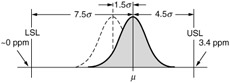
   Figure 12.24: A process with a 1.5-sigma shift to the right.

Given that the process mean might be as far as 1.5 ƒ from the target and that a product is made up of many parts, a 3-sigma process might not be as good as we originally stated. Just how good is it?

Suppose that a product is made up of m parts. We will calculate the probability that all m parts are within specifications when the process mean is 1.5 ƒ above the target and the distance from the target to either specification limit is k ƒ . That is, we are considering a k-sigma process with a process mean off center by an amount 1.5 ƒ . Let X be the measurement for a typical part, and let p be the probability that X is within the specification limits; that is, p = P (LSL < X < USL). If p _m is the probability that all m parts are within the specification limits, then assuming that all parts are identical and probabilistically independent, the multiplication rule for probability implies that p _m = p ^m .

To calculate p = P (LSL < X < USL), we need to standardize each term inside the probability by subtracting the process mean ¼ and dividing the difference by ƒ . Let T be the target. Then we have LSL = T - k ƒ and USL = T + k ƒ (because the process is a k-sigma process) and ¼ = T + 1.5 ƒ (because the mean has shifted upward by an amount 1.5 ƒ ). Therefore, the standardized specification limits are

This implies that

p = P ( -k -1.5 < z < k - 1.5) = P ( z < k - 1.5) - P ( z < -k - 1.5)

When this is actually carried out with a software package, one finds that for many applications a 3-sigma process is inadequate, having about 7% of its individual parts out of specifications. In contrast, a 6-sigma process is extremely capable, with only 0.34% of its 1000-part products out of specifications. No wonder Motorola's 5-year goal (as of 1992) was to achieve "6-sigma capability in everything we do." This is remarkable quality! The concept of the 6-sigma quality is shown in Figure 12.25.

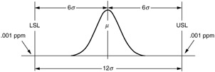
Figure 12.25: A process with potential capability of 12 sigma equaling the tolerance.

The above analysis shows how we can calculate the capability of a process if we know that it is a k-sigma process for any specific k. We conclude this section by asking a slightly different question. If a company has produced many parts and has observed a certain fraction to be out of specifications, what is their estimated value of k? For example, suppose that after monitoring thousands of gaskets produced on its machines, a company has observed that 0.545% of them are out of specifications. Is this company's process a 3-sigma process, a 4-sigma process, or what?

To answer this question, we assume a worst-case scenario in which the mean is above the target by an amount 1.5 ƒ . Then, from the above equation, we know that the probability of being within specifications is

p = P ( Z < k - 1.5) - P ( Z < -k - 1.5)

if the process is a k-sigma process. However, we now know p from observed data, and we want to estimate k. This can be done with many software packages. In this case, it turns out that the value of k is 4.077.