MACHINE CAPABILITY ANALYSIS USING CAPABILITY FORMS

This section reviews the use of capability analysis sheets for the purpose of determining machine capability. The forms used, and in fact the procedure itself, are extremely similar to other forms used throughout process industries; and the basic procedure employed with these other forms is identical.

Some of the important considerations in conducting a machine capability analysis are:

• Thirty or more consecutive units should be run and measured. Whenever possible and economical, use more than 30 items.

• All gauges employed in the analysis should be properly calibrated. When possible, only one gauge (with known inherent variability) should be used during the study. This procedure will avoid the introduction of nonmachine (false) variability.

• All adjustments should be made before, but not during, the process test run.

• Whenever possible, the units should be measured at a measurement level that allows at least 10 data categories within the specification limits. For example, if the specification was ±.003, giving a range of .006, the data should be taken to the nearest .0005, dividing the .006 range into 12 categories (as close to 10 as this example allows). When data are available at a greater level of precision, they should be recorded at that level and grouped at a later time.

• To make use of this procedure, the process distribution should be normal.

• The individual measurements should be recorded in the sequence that they were produced.

• All test units should be identified by sequence number and retained for future diagnostic use; this is especially important should the process be shown to be not capable.

To review the procedure necessary to conduct a study of this type, we offer an example of a capability study conducted for a machined shaft diameter. The engineering specification for this shaft was 1.010 ± 0.005" 1 equivalent to 1.005 to 1.015. Thirty initial pieces were run and measured, with the measures recorded to the nearest 0.001". The steps used in the analysis follow:

• Step 1: Collect and record the data on an appropriate form (see Figure 12.10).

  
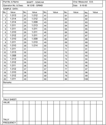
  Figure 12.10: Collection of data for a machine capability study.

• Step 2: Tally and develop a frequency distribution for the recorded data (see Figure 12.11).

  
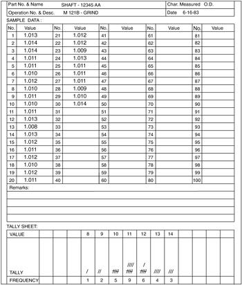
  Figure 12.11: The tallied frequency distribution of the shaft example.

• Step 3: Transcribe the data onto a capability analysis sheet (see Figure 12.12).

  
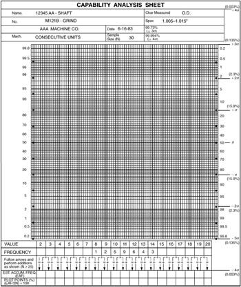
  Figure 12.12: Data transferred onto the capability analysis sheet.

• Step 4: Complete the EAF (estimated accumulated frequency) row. For the first (left-most) entry, transcribe the frequency to the EAF cell directly below it (see Figure 12.13a).

  
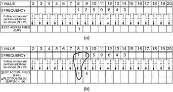
  Figure 12.13: The generation of the EAF.

  For each additional cell (following the sequence of arrows, add the previous EAF + previous frequency + current frequency to obtain the current EAF (see Figure 12.13b). For example, the EAF corresponding to the second frequency is determined as follows :

  EAF2	=	EAF1 + F1 + F2
  	=	1 + 1 + 2
  	=	4

  Continue to complete the remainder of the EAF row. To check whether the calculations are correct, add the final frequency to the final EAF. The sum value should equal N x 2 .

• Step 5: Complete the plot points (%) row.

  To calculate the plot points for each value, divide each EAF by 2N (double the sample size ), and multiply the result by 100. This procedure has the effect of estimating the cumulative percentage of the process distribution at the midpoint of each value class.

  As an example, the first value class has an F value of 1; therefore,

  1/60 — 100 = 1.67% = 1.7% = plot point

  Following this method, we can generate all the plotting points.

• Step 6: Locate and mark the plot points on the graph (see Figure 12.14).

  
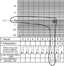
  Figure 12.14: Plotting the points on the graph paper.

• Step 7: After all points have been plotted, draw a line of best fit through the points. (Note: You are looking for a straight line, because the normal distribution plotted in a probability paper is always a straight line. If, after drawing the line of best fit, the points off the line appear to have a pattern [such as curving to the right at the top of the graph], you should note that the distribution is not normal, which means that this procedure should be discontinued; and the evidence of nonnormality may be a result of assignable causes in the process that could jeopardize its potential for capability.)

  Make sure then that the line of best fit extends far enough to cross the ±3 sigma and the ±4 sigma limits at the top and bottom of the analysis sheet.

• Step 8: Draw the upper and lower specification values on the graph (use dashed lines).

• Step 9: Record the ±3 sigma limit value and the ±4 sigma limit values in the upper right-hand corner of the analysis sheet. These values are found by identifying the point at which the line of best fit crosses each of the appropriate horizontal sigma lines and rounding to the level of precision used (in this case, 0.001").

• Step 10: Interpret for process capability.