CAPABILITY ANALYSIS USING THE EXPONENTIAL DISTRIBUTION

Some manufacturing processes have variation that is completely one sided. These processes may best be modeled by the exponential distribution (see Figure 14.2C). Some typical examples are measurements of transistor saturation voltage, total indicated runout (TIR), cutoff lengths, molded wall thickness , trimmed resistor values, and magnetic flux density.

The data in Figure 14.9 were collected from a stable cutoff process and follow the shape of the exponential distribution.

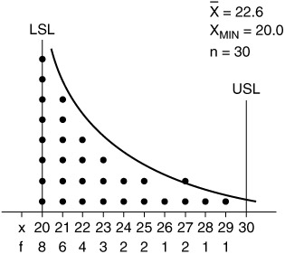
Figure 14.9: Exponential distribution with the associated data.

In this case, the use of ±3 or ±4 standard deviations and the density of the normal distribution are irrelevant to the study of capability. The exponential distribution is asymptotic to both the horizontal axis and to a minimum value. The minimum value is called the origin parameter. The density function of the exponential distribution assumes that the origin parameter equals zero. In addition, the mean of the exponential distribution does not divide the distribution into two equal halves . About 36.8% of the exponential curve is above the mean, and about 63.2% is below.

ANALYZING EXPONENTIAL DISTRIBUTIONS

First, transform the measurement scale so that the origin parameter equals zero(0). Some measured characteristics follow the exponential distribution and have zero as the most frequent and minimum value ( X _MIN ). Measurements of TIR, parallelism, and concentricity all have zero as a minimum possible value.

All other values are greater than zero. In these cases, when zero is also the most frequent measurement, the measurement scales does not require transformation. The origin parameter already equals zero.

Other measured characteristics follow the exponential distribution but do not have zero as the minimum and most frequent value. In these situations, the minimum value must be subtracted from all of the numbers on the measurement scale. By subtracting the minimum value from itself, the origin parameter is made equal to zero. Figure 14.10 shows the original measurement scale and a transformed scale for the cutoff process data.

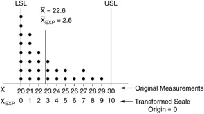
Figure 14.10: Original measurement scale and transformed scale.

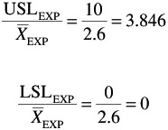
The next step in analyzing exponential distributions is to calculate a standardized ratio for the specifications. A standardized ratio X / is used to calculate the area under the exponential curve. The ratio is calculated for values from the transformed measurement scale. A standard ratio must be calculated for each specification limit.

The third step is to calculate the area above the standardized ratio. The area under the exponential distribution and above a standardized ratio is defined by the natural antilogarithm of the standardized ratio ( e ). This is the same as raising e ( e = 2.7182818) to the negative power of the standardized ratio (see Figure 14.11).

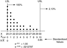
Figure 14.11: The area under the exponential distribution and above a standardized ratio.

Use the procedure shown in Figure 14.12 to calculate the natural antilogarithm by using the Sharp series of scientific calculators . The area below the lower specification limit (LSL) is calculated by subtracting the area above the LSL from 1.0.

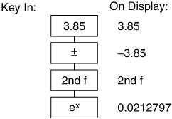
Figure 14.12: Procedure to calculate the natural antilogarithm with the use of the Sharp Series scientific calculators.