Understanding IP Routing

EXAM 70-293 OBJECTIVE 2, 2.1.2, 3

The basic concept of routing is that each packet on a network has a source address and a destination address. These two addresses are stored in the packet’s header information. That means that any device on the network that receives this packet can inspect the header to find out where the packet came from and where it’s going. If we provide our device with a little more information, such as details concerning the network’s design and implementation, that device can also change the routing for the packet in an intelligent manner to help lower the total cost of the traffic.

So that we’re all on the same page, we need to start by reviewing the basics of routing. Keep in mind as we go through the following material that it is mainly review and not intended as the final word on these topics.

Reviewing Routing Basics

Understanding the concepts concerning IP addressing is critical to understanding how IP routing works. A good understanding of IP addressing, and subsequently the art of subnetting, requires that you be comfortable with binary notation and math.

You already know that an IP address is a numeric identifier assigned to every machine on a network. This address tells where the device is located on the specific network.

Exam Warning

Keep in mind that an IP address is a software address. Don’t confuse it with a hardware address. The hardware address is hard-coded into the machine itself or in the network interface card (NIC). Also keep in mind that starting with Windows 2000, Microsoft began listing IP address ranges in the same manner that Cisco does. This method, Classless Interdomain Routing (CIDR), lists the IP address followed by the number of ones in the subnet mask. For instance, 192.168.1.0 with a subnet of 255.255.255.0 is written as 192.168.1.0/24.

As a quick review, IP addresses are currently made up of 32 bits of information. These bits are divided into four sections (octets) that each contains 1 byte (6 bits). You will see IP addresses specified in three basic formats:

• Binary such as in 11000000.10101000.00000000.00000001

• Dotted-decimal such as in 192.168.0.1

• Hexadecimal such as in C0 A8 00 01

All three of these examples represent the same IP address. In reality, the computer can use only the binary version. The other two formats are provided because they are easier for people to understand and use.

There are three basic types of IP addresses:

• Unicast addresses IP addresses assigned to a single network interface that is attached on the network. Unicast IP addresses are used for one-to-one communications between hosts.

• Broadcast addresses IP addresses designed to be received and processed by every IP address located on a given network. They’re basically one-to-many communications.

• Multicast addresses IP addresses where one or more IP nodes can listen in on the same network segment. Multicast IP addresses are also one-to-many communications.

Next, you should also understand the differences between routed and Network Address Translation (NAT) connections. NAT is the process of switching back and forth between the IP addresses used on an internal network, sometimes referred to as private addresses, and Internet IP addresses, sometimes known as public addresses.

There are three address blocks set aside and defined as private address space:

• 10.0.0.0 with a subnet mask of 255.0.0.0, or 10.0.0.0/8 This network is a private address space that has 24 host bits that can be used.

• 172.16.0.0 with a subnet mask of 255.240.0.0, or 172.16.0.0/12 This network is a private address space that has 20 host bits that can be used. This provides a range of 16 class B network IDs from 172.0.0.0/16 through 172.31.0.0./16.

• 192.168.0.0 with a subnet mask of 255.255.0.0, 192.168.0.0./16 This network is a private address space that has 16 host bits that can be used. This provides a range of 256 class C network IDs from 192.168.0.0/24 through 192.168.255.0/24.

Remember that private and public spaces do not overlap. Machines on an intranet with a private IP address cannot directly connect to the Internet. Instead, they must be connected indirectly via either a proxy server of NAT. Essentially, all of the computers on your intranet are masquerading behind a single public IP address.

Exam Warning

Understand the ranges and subnet masks used with private addressing. Know how NAT translates and connects for them.

Routed connections require a single public IP address for each connection to the Internet. Using NAT allows you to connect multiple private addresses to a single public IP address. This is done by translating and modifying packets to reflect the changed addressing information.

There are three basic components that make up NAT:

• Translation This component maintains the NAT table for inbound and outbound connections.

• Addressing This component is handled by a stripped-down version of a Dynamic Host Configuration Protocol (DHCP) server that assigns the IP address, subnet mask, default gateway, and IP address of the Domain Name System (DNS) server.

• Name resolution This component forwards all name-resolution requests to the DNS server defined on the Internet-connected adapter, and then returns the reply. It can be thought of as a DNS proxy.

  Exam Warning

  Understand the three components of NAT and how they interact with other Windows Server 2003 components such as DNS and DHCP.

Keep in mind that NAT is not always the solution. It is extremely limited when it comes to security. You cannot encrypt anything that is carrying or that has been derived from an IP address. Tracking hackers and other problems is also extremely difficult, because the source IP address is stripped away in the NAT process. Another problem arises when you try to use NAT with large networks that have many hosts attempting to communicate with the Internet at the same time. The size of the mapping tables in this kind of environment is overwhelming and can cause performance problems.

Another basic concept related to IP routing is how the Internet Control Message Protocol (ICMP) works. ICMP is a maintenance protocol used to create and maintain routing tables. It supports router discovery and advertisements to hosts on a network. Very simply, its designed to pass control and status information between TCP/IP devices. When a client computer starts up on your network, it usually has only a few entries in its routing table. When that host sends data out to a specific destination on a network, the host first checks its routing table to see if there is already an entry matching the destination’s IP address. If no match is found, the packet is sent to the default gateway. When the default gateway receives the packet, it will check to see if it has a matching entry in its routing table. If it does, it forwards the packet to the destination. At the same time, it sends an ICMP message back to the originating host, telling that host about the better route available. ICMP can also let hosts on a network know if a specific router is still active by sending out periodic messages with this kind of information.

Head of the Class...
IP version 6

The Internet that we have all come to know and love uses IP version 4 (IPv4) and is based on 32-bit addressing. Because of the numerous disadvantages of IPv4, including the problem of limited address space that NAT addresses, a new proposal was put forth in 1995. Originally called Internet Protocol Next Generation (IPng), this proposal offered several improvements, including 128-bit addressing, global addressing, automatic configuration, built-in security, improved quality of service (QoS) support, and built-in mobility. The new version of IP became known as IP version 6 (IPv6). IP version 5 was reserved for a different proposal that was never adopted or implemented.

Because of the differences between IPv4 and IPv6, IPv6 is not backward-compatible with IPv4. The address syntax is just one example. IPv4 addresses can be expressed in the traditional 192.168.0.0/20 format. IPv6 has been forced to settle on the colon-hexadecimal notation. The 128-bit block is divided into eight 16-bit blocks and delimited by colons. The 32-bit block of IPv4 is divided into four 8-bit blocks.

An example of an IPv6 unicast address is 3FFE:FFFF:2A:41CD:2AA: FF:FE5F:47D1. Leading zeros within a block are suppressed, but each block must contain at least one hexadecimal digit. Another example is FE80:0:0:0:2AA: FF:FE5F:47D1. Notice the 0 blocks. IPv6 allows for the compression of IPv5 addresses using double colons. The above address then becomes FE80::2AA:FF:FE5F:47D1. A multicast address such as FF02:0:0:0:0:0:0:1 would then become FF02::1.

IPv6 doesn’t use subnet masks, but rather continues to use the CIDR notation. Using this notation, 3FFE:FFFF:2A:41CD::/64 would be a subnet identifier; 3FFE:FFFF:2A::/48 would be a route; and FF::/8 would be an address range.

Just remember that IPv6 is actually a suite of protocols. It replaces IP, ICMP, Internet Group Management Protocol (IGMP), and Address Resolution Protocol (ARP) in the TCP/IP protocol suite.

Routing Tables

A routing table is basically a list, a huge list sometimes, that is used to direct traffic on a network. The table includes information about what other networks are reachable from a given network by providing the network address and subnet mask, as well as the metric, or cost, for that specific network route. Another way to think of it is as a database of routes to other locations.

The way this works is simple. When a packet arrives at the routing device (which could be a dedicated router or a Windows Server 2003 computer), the routing table is queried to discover the lowest cost route to the intended destination. Sometimes when there is no specific information concerning that network in the routing table, the packet will be forwarded to the default gateway, assuming that the default gateway will get the packet where it needs to go.

The level of detail, or the number of routes in the table, depends on whether the IP node is a host or a router. Usually, a host will have fewer entries in this table than a router has in its table. For instance, it would be normal to find an IP host configured with a default gateway. Creating a default route in the table allows for the effective summarization of all destinations. Routing tables on a router, on the other hand, will normally contain an entry for each and every reachable network on the IP network system.

Let’s turn our attention back to the table itself. Each of the rows in this list, or entries in this database, is commonly referred to as a route. There are three basic types of routes:

• Host route A route to a specific IP address in the network. A host is a particular computer, or more specifically, an interface on a computer or device. In these cases, the network mask is always 255.255.255.255 (/32). Host routes are typically used for custom routes to specific hosts. This helps in the optimization and control of a network.

• Network ID route A route for classful, classless, subnet, and supernetted destinations. The network mask in these cases will be somewhere between 129.0.0.0 (/1) and 255.255.255.254 (/31).

• Default route A route to all other destinations. This route is used when the routing table cannot find a host or network ID route that matches the destination in the packet’s header. The default route has a destination of 0.0.0.0 and a network mask of 0.0.0.0 (/0), and it is sometimes expressed as 0/0. All destinations not found in the routing table are simply forwarded to this destination, where the specific destination address will be found.

Each route in the routing table contains the necessary forwarding information for a range of destination IP addresses. This information includes two values for the destination IP address: the next-hop interface and the next-hop IP address. The next-hop interface is just a representation of the next physical or logical device over which the IP packet will be forwarded. The next-hop IP address is the IP address of the node to which the IP packet is being forwarded. In an indirect delivery, the next-hop IP address is the IP address of a directly reachable intermediate router to which the packet is being forwarded.

So, from this discussion, we glean that there is enough information contained in the route entry of a routing table to identify the destination, the next-hop interface, and the next-hop IP address, and to determine which route is the best when there is more than one route available to the intended destination. Let’s break down the route entry into its component parts:

• Destination Sometimes referred to as the network destination, this value is usually a representation of the IP address that is reachable with this route. It is usually used in conjunction with the Network Mask field. This can be a network ID (classful, subnet, or supernet) or an IP address. Other terms that are sometimes used to represent the destination include destination host, subnet address, network address, and default route. The destination for a default route is 0.0.0.0. The destination for a limited broadcast is 255.255.255.255.

• Network Mask Sometimes referred to as the netmask, this value is a bit mask that is used to determine the significant bits in the Destination field. The 1 bit in a network mask identifies those bits that must match the Destination field for this route. The 0 bit indicates the bits that don’t need to match the Destination field. This field is usually a string of contiguous 1 bits followed by a string of contiguous 0 bits. The combination of the destination and the network mask defines a range of IP addresses. A host route has a network mask of 255.255.255.255. With this mask, only an exact match with the destination would be able to use this route. On the other end of the spectrum, a default route has a network mask of 0.0.0.0. A mask of 0.0.0.0 allows any destination to use this route. A subnet or network route has a mask that exists somewhere between these two extremes.

• Next-hop IP Address This points to the IP address where the packet is to be forwarded using this route. It’s sometimes also referred to as the forwarding address and most often called the gateway. This gateway must be directly reachable by this router by using the interface defined in the Interface field. This can be a hardware address, a network address, or sometimes even the address of the interface attached to the network.

  Note

  When working with routes of directly attached network segments, the Next-hop IP Address field can be set to the IP address of the network segment’s interface. This is the default behavior of the IP routing table for the Windows 2003 Server family.

• Interface This is the logical or physical interface used when forwarding the packet using this specific route. It indicates the local area network (LAN) or demand-dial interface needed to reach the next router. The value here can be either a logical name or the IP address assigned to the interface. This can be the port number or some other logical identifier.

  Note

  Windows Server 2003 family uses the IP address assigned to the interface.

• Metric This field is where the route’s cost is maintained. It’s commonly used to store the hop count, or the number of routers between the host and the destination. It is also used by the route-determination process to choose among the many routes to the same location that might be possible. When there are multiple routes with the same destination and network mask, the route with the lowest metric value is used. Anything on the local subnet is always considered one hop. Each router crossed is counted as an additional hop. The lowest metric is usually the preferred one.

• Protocol This field shows how the route was learned. This column will normally list RIP, OSPF, or other routing protocols. If it lists Local, the router is not receiving routes.

Configuring & Implementing...
Viewing Routing Tables

Viewing your routing tables in Windows Server 2003 is a simple procedure, but you must be logged on as an Administrator or, as a security best practice, using the Run As command. Follow these steps:

1. Select Start | Control Panel | Administrative Tools | Routing and Remote Access.

2. In the console tree on the left side of the Routing and Remote Access window, click the plus sign to the left of Routing and Remote Access.

3. Under that, you will see the name of the server. Click the plus sign there, and you’ll see IP Routing.

4. Click the plus sign next to IP Routing, and you should see Static Routes.

5. Right-click Static Routes and choose Show IP Routing Table from the context menu.

   You can also use a command-line utility to view the routing table. (Speed is one of the most important reasons for choosing to use the command line over a GUI tool.) To view the routing table from the command prompt, click Start | All Programs | Accessories | Command Prompt. This opens the command prompt window. At the prompt, type route print and press the Enter key. You’ll now see a screen resembling the one shown in Figure 4.1.

   
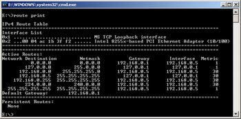
   Figure 4.1: Viewing the Routing Table from the Command Prompt

The routing table shown in Figure 4.2 (viewed from the Windows Server 2003 Routing and Remote Access utility) is for a computer running Windows Server 2003 Enterprise Edition with one 10MB network adapter, an IP address of 192.168.0.13, a subnet mask of 255.255.255.0, and a default gateway of 192.168.0.1.

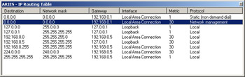
Figure 4.2: IP Routing Table

Let’s look at the individual rows more closely:

• The first row in the table, beginning with 0.0.0.0, is the default route.

• The second and third rows, beginning with 127.0.0.0 and 127.0.0.1, are the loopback network.

• The fourth row, beginning with 192.168.0.0, is the local network.

• The fifth row, beginning with 192.168.0.13, is the local IP address.

• The second-to-last row, beginning with 224.0.0.0, is the multicast address.

• The final row, beginning with 255.255.255.255, is the limited broadcast address.

We’ll now turn our attention to the upkeep of these tables. You can perform the maintenance of the routing tables manually or automatically. If you do it manually, you’ll be using static routing. If you do it automatically, you’ll be using dynamic routing. Let’s take a closer look at these two concepts.

Static versus Dynamic Routing

Remember that the basic idea of routing is that each packet you find on your network has a source and a destination. That means that any device that receives the packet inspects the packet’s headers to determine where it came from and where it’s going. When the device has information about the network, such as how long it would take a packet to go from one point to another, that device can change the routing intelligently to improve the performance of the network.

Static routing uses manually configured routes. Here, there is no attempt to discover other routers or systems on a network. All entries into the routing table are entered by hand, and the routing table is used to get information to other networks. This type of routing works well with classless routing, because each route must be added with a network mask. It works well for small networks, but it doesn’t scale well. Static routes are often used to connect to the Internet. Static routing is, however, not fault tolerant. Figure 4.3 shows a simple network using static routing.

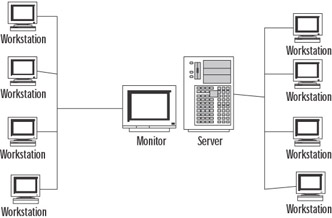
Figure 4.3: Simple Network Using Static Routing

Dynamic routing doesn’t depend on fixed, unchangeable routes to remote networks being added to the routing tables. In other words, you don’t need to enter the routes by hand. Dynamic routing uses routing protocols to maintain the routing tables. Dynamic routing allows for the discovery of the networks surrounding the router by finding and communicating with other nearby routers in the network. Routes are discovered using routing protocol traffic and are then added or removed from IP routing tables as required. Dynamic routing can provide fault tolerance. When a route is unreachable, the route is removed from the routing table. Figure 4.4 shows a more complex network using dynamic routing.

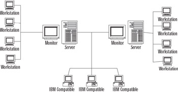
Figure 4.4: A More Complex Network Using Dynamic Routing

In summary, static routing has two main advantages:

• It works well with classless routing.

• It works well with small networks.

Static routing also has two main disadvantages:

• It doesn’t scale well.

• It is not fault tolerant.

For more complex networks, dynamic routing offers several advantages:

• It scales well with larger organizations.

• It is fault tolerant.

• It requires less administration than static routing.

Gateways

Although we’ve mentioned the term default gateway earlier in this chapter, we have not really gone into much detail about what a gateway is. Basically, a gateway is a device that connects networks using different communication protocols in a way that allows for information to pass from one network to the other. It both transfers and converts the information into a form that can be used by the protocols on the receiving network. Think of it as a TCP/IP node that has routing capabilities. In other words, a gateway is a kind of router. A router, by definition, is a device or computer that sends packets between two or more network segments as necessary, using logical network addresses, most often IP addresses. The default gateway is the path used to pass information when the device doesn’t know where the destination is. More directly, a default gateway is a router that connects your host to remote network segments. It’s the exit point for all the packets in your network that have destinations outside your network.

Configuring & Implementing…
Planning a Routing Strategy for IP Multicast Traffic

EXAM 70-291 OBJECTIVE 3.1.2

Multicast traffic involves sending a message to multiple devices using a single (multicast) IP address. Multicasting is referred to as point-to-multipoint communication because the sender only has to send the message to one address to a group of computers that share a multicast group ID, which is an address from the Class D range.

Planning a Windows Server 2003 routing strategy in which multicast messages are sent involves the following steps:

1. Planning for the deployment of MADCAP servers (Multicast Address Dynamic Client Allocation Protocol). MADCAP is part of the Windows Server 2003 DHCP service, but works independently of DHCP.

2. Planning for deployment of routers that support IP multicasting. The routers need to be configured to use multicast routing protocols. Windows Server 2003 does not include multicast routing protocols, but RRAS supports multicast routing protocols such as Protocol Independent Multicast (PIM), Multicast Extensions to OSPF (MOSPF) and Distance Vector Multicast Routing Protocol (DVMRP).

3. Configuring the Internet Group Management Protocol (IGMP).

4. Configuring Multicast scopes on the MADCAP server, using administrative scoping for multicast addresses that are used on the internal network and global scoping for multicast addresses that are used on the Internet.

5. Configuring client computers to be MADCAP clients.

New & Noteworthy...
Multiple IP Addresses

Computers running Windows Server 2003 can have multiple IP addresses, even if the computer has only one NIC. In this case, if your network is divided into multiple logical IP network subnets, you can set up the single NIC to have multiple IP addresses. Then the address 192.168.0.10 could be used to communicate with the workstations and computers you have on the 192.168.0.0 subnet, and the address 192.168.1.10 could be used to communicate with the workstations and computers you have on the 192.168.1.0 subnet.

Keep in mind that if you are using a single NIC, the IP addresses must be assigned to either the same network segment or to segments that are part of the same single logical network. If your network is divided into multiple physical networks, you will need to use multiple NICs, with each card assigned an IP address from the different physical network segments.

Configuring & Implementing...
Configuring Multiple Gateways

To install multiple gateways, follow these steps:

1. Select Start | Control Panel | Network Connections, and then select the connection you want to configure.

2. Click Properties and double-click Internet Protocol (TCP/IP) to open the Internet Protocol (TCP/IP) Properties dialog box, shown in Figure 4.5.

   
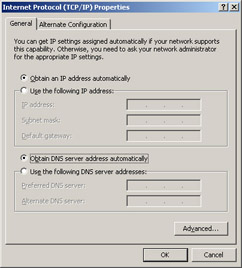
   Figure 4.5: Internet Protocol (TCP/IP) Properties

3. Click the Advanced button to open the Advanced TCP/IP Settings dialog box, shown in Figure 4.6.

   
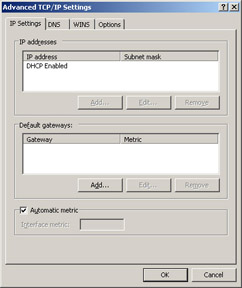
   Figure 4.6: The IP Settings Tab of the Advanced TCP/IP Settings

4. On the IP Settings tab, you can add default gateways as you deem necessary. Click the Add button, and then type the gateway address in the Gateway text box, as shown in Figure 4.7.

   
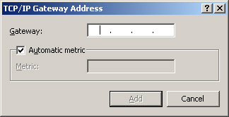
   Figure 4.7: Enter the Gateway Address

5. The metric, as we have discussed previously, provides a relative cost of using this gateway, or route. When multiple gateways are available for a particular IP address, the gateway with the lowest metric will be used. If for some reason the Windows Server 2003 computer cannot communicate with the first gateway, it will try to use the gateway with the next lowest metric. By default, Windows Server 2003 assigns the metric to the gateway automatically. If you want to do so manually, uncheck the Automatic metric check box and enter a metric in the text box.

Routing Protocols

EXAM 70-291 OBJECTIVE 3.1.1

Router discovery enables new, or rebooted, routers to configure themselves automatically. The two major and most common dynamic-routing protocols are RIP and OSPF. Both of these protocols are supported by the Windows Server 2003 family. Both are interior gateway protocols (IGPs) that use routers to communicate (not to be confused with the proprietary Cisco IGRP). But before we discuss these two protocols, we need to explore how protocols make routing decisions.

In general, routing protocols can use one of two different approaches to making routing decisions:

• Distance vectors A distance-vector protocol makes its decision based on a measurement of the distance between the source and the destination addresses.

• Link states A link-state protocol bases its decisions on various states of the links that connect the source and the destination addresses.

Distance-vector algorithms, also known as Bellman-Ford algorithms, periodically pass copies of their routing tables to their immediate network neighbors. The recipient adds what is called a distance vector, which is little more than a distance value, to the routing table it has just received, and then forwards it on to its immediate neighbors. The process results in each router learning about the other routers and thereby developing a cumulative table of network distances to other routers. This table is then used to update the router’s own routing table. Keep in mind that the only thing the router learns about is distance.

The main drawback to distance-vector routing is that it requires time for the changes in a network to propagate across the network. This makes distance-vector routing inappropriate for larger, more complex networks. The advantages of distance-vector routing are its ease of configuration, use, and maintenance. As we will discuss shortly, RIP is the epitome of distance-vector routing.

Link-state routing algorithms are usually known cumulatively as shortest path first (SPF) protocols. OSPF, which will be discussed shortly, is an example of this protocol group. These protocols maintain a complex database that describes the network’s topology. Link-state protocols develop and maintain extensive information concerning the network’s routers and how they interconnect. They do this by exchanging link-state advertisements (LSAs) with each other. Any change in the network will trigger the exchange of LSAs. Each router then constructs an extensive database using these received LSAs, so it can compute different routes and determine how reachable the networked destinations really are. This information is then used to update the routing table. Component failures and growth of the network are easily documented.

The main drawbacks to using link-state protocols involve the heavy use of bandwidth, memory, and processor time. Especially during the initial discovery process, link-state protocols flood the network with messages, thereby lowering the overall network efficiency. Also, overall, link-state protocols require more memory and higher processor speeds than distance-vector protocols need for efficient operation.

The main advantage of link-state protocols comes into play with large and complicated networks. A well-designed network will be more able to withstand the effects of unexpected changes using link-state protocols. Overhead caused by the frequent, time-driven updates required for distance-vector protocols can be avoided. Networks using a link-state protocol are also more scalable. For most large networks, the advantages of using link-state protocols will outweigh the disadvantages.

RIP

RIP is simple and easy to configure and is used widely in small and medium-sized networks. RIP is an IGP used to route data within autonomous networks. RIP does have performance limitations, however, that restrict its usefulness on medium-sized to large networks. RIP is a distance-vector routing protocol. This means that it distributes routing information in the form of a network ID and the number of hops (or the distance) from the destination. RIP has a maximum distance of 15 hops. Anything over that is considered unreachable.

There are two versions of RIP: version 1 described in RFC 1058 and version 2 described in RFC 1723. Windows Server 2003 supports both RIP versions.

RIP version 1 is a class-based routing protocol. Only the network ID is announced here. The message format for RIP version 1 is shown in Figure 4.8.

Figure 4.8: RIP Version 1 Message Format

RIP version 2 is a classless routing protocol. This version includes both a network ID and a subnet mask in its announcement. It also provides more information, allowing for both authentication and a measure of security. The message format for RIP version 2 is shown in Figure 4.9.

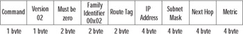
Figure 4.9: RIP Version 2 Message Format

There are several shortcomings to RIP version 1:

• RIP version 1 uses MAC-level broadcasting, requiring all hosts on a network to process all packets.

• RIP version 1 doesn’t support sending a subnet address with the route announcement. This can be a problem when there is a shortage of available IP addresses.

• Because RIP version 1 route announcements are being addressed to the IP subnet and MAC-level broadcast, non-RIP hosts may also be receiving the RIP announcements, contributing to the broadcast clutter and possibly lowering the efficiency and performance of your network.

• By default, every 30 seconds, RIP routers broadcast lists of networks they can reach to every other adjacent router. Again, this can contribute to lower network performance.

• RIP version 1 does not handle subnetted addresses well, since it doesn’t send the subnet address along with the broadcast.

• RIP version 1 provides no defense from a rogue router. A rogue router is an RIP router that advertises false or erroneous route information.

• RIP version 1 is difficult to troubleshoot. In general, most problems in RIP routing stem from incorrect configuration or from the propagation of bad routing information.

So, what does RIP version 2 do to attempt to correct the problems with RIP version 1?

• RIP version 2 advertisements include the subnet mask with the network ID.

• RIP version 2 sends multicast announcements to the multicast IP address 224.0.0.9 with a time to live (TTL) of 1 instead of broadcasting announcements, so it does not require IGMP.

• RIP version 2 allows for authentication to substantiate the source of the incoming routing announcements.

• RIP version 2 is compatible with RIP version 1.

RIP routers begin with a basically empty routing table and start sending out announcements to the networks to which they’re connected. These announcements include the appropriate routes listed for all interfaces in the router’s routing table. The router also sends out a RIP General Request message asking for information from any router receiving the message. These announcements can be broadcast or multicast. Other routers on other networks hear these announcements and add the original router and its information to their own routing tables. They then respond to the new router’s request for information. The new router hears the announcements from these other routers on the network and adds them and their information to its own routing table.

After the initial setup, the RIP router will send out information based on its routing table. The default time period is 30 seconds. Over time, the routers of the network develop a consensus of what the network looks like. The process of developing this consensual perspective of the network’s topology is known as convergence. Basically, this means that the network’s routers individually agree on what the network looks like as a group. It is this very process of convergence, however, that can sometimes lead to problems. A typical network using convergence is shown in Figure 4.10. One of the occasional problems that occurs is called counting to infinity. Let’s look at how that happens.

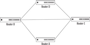
Figure 4.10: Typical Network Using Convergence

In our example, we will assume that Router A has failed. With its failure, all the hosts on the A network will no longer be accessible from the other three networks. After missing six updates from Router A, Router B will invalidate its B–A route and advertise its unavailability. Routers C and D remain ignorant of the failure of Router A until notified by Router B. At this point, both Router B and Router D still think they can get to Router A through Router C, and they raise the metric of this route accordingly. So, Routers B and D send their next updates to Router C. Router C, having timed out its route to Router A, still thinks it has access through Router B or Router D. Thus, a loop is formed between Routers B, C, and D, based on the mistaken belief that both Routers B and C can still access Router A. With each iteration of updates, the metrics are incremented an extra hop for each route. This count speeds up the process by which the router approaches its definition of infinity—the point where the router says the destination is unreachable.

There are two methods of preventing this counting to infinity loop: split horizon and triggered updates. If the router is implementing split horizon, routes will not be announced back over the interfaces by which they were learned. The limitation of the split-horizon approach is that a route will not timeout until it has been unreachable for six tries, so each router has five opportunities to transmit incorrect information to the neighboring routers. If the router is implementing split horizon with poison reverse, routes learned on interfaces are announced back as unreachable. Split horizon with poison reverse is much more dependable than simple split horizon. However, although split horizon with poison reverse will stop loops in small networks, loops are still possible on larger, multipath networks.

Fault tolerance in RIP networks is based on the timeout of RIP-learned routes. When changes happen in the network, RIP routers send out triggered updates, rather than waiting for a scheduled time for routing announcements. These triggered updates contain the routing update and are sent immediately. Triggered updates are nothing more than a method of speeding up split horizon with poison reverse. However, triggered updates are not foolproof. While the triggered updates are being propagated around the network, routers that have not received the triggered update are still sending out the incorrect information. It’s possible that a router could receive the triggered update and then receive an update from another router reintroducing the incorrect information, so the count-to-infinity problem, though not as likely, is still possible.

OSPF

Because OSPF is designed to work inside the network area, it belongs to a group of protocols called IGRPs. OSPF is defined in RFC 2328 and its purpose is to overcome the shortcomings of both versions of RIP when they are used for large organizations. OSPF is designed for use on large or very large networks. OSPF is much more efficient than RIP, and it also requires much more knowledge and experience to set up and administer.

There are many reasons why OSPF is a better choice for large networks than either version of RIP, including the following:

• Faster detection and changes of the network topology. This means less chance of encountering the count-to-infinity problem.

• OSPF routes are loop-free.

• In OSPF, large networks can be broken down into smaller contiguous groups of networks, called areas. (RIP does not allow for the subdivision of a network into smaller components.) Routing table entries can then be minimized by using the technique called summarizing. Summarizing allows for the creation of default routes for routes outside the area.

• The subnet mask is advertised with OSPF. This provides support for disjointed subnets and supernetting.

• Route exchanges between OSPF routers can be authenticated.

• Because external routes can be advertised internally, OSPF routers can calculate least-cost routes to external destinations.

The packet header structure for OSPF is shown in Figure 4.11.

Figure 4.11: The OSPF Packet Header Structure

There are five basic messages that are attached to this header structure:

• Hello packet Used to discover and maintain information about neighboring routers.

• Database Description packet Used to summarize database contents.

• Link-State Request packet Used to initialize the database download from another router.

• Link-State Update packet Used to update other routers with the information contained in the local router’s database.

• Link-State Acknowledgment packet Used to acknowledge flooding of information from other routers.

OSPF is a link-state routing protocol that uses LSAs to send information to other routers in the same area, known as adjacencies. Included in the LSA is information about interfaces, gateways, and metrics. OSPF routers collect this information into a link-state database (LSDB) that is shared and synchronized among the various routers. Using this database, the various routers are able to calculate the shortest path to other routers using the SPF algorithm. The cost of each router interface is assigned by the network administrator. This number can include the delay, the bandwidth, and any monetary cost factors. The accumulated cost of any OSPF network can never be more than 65,535. So, the way OSPF works can be divided into three main phases:

• The LSDB is put together from neighboring routers.

• The shortest path to each node is then calculated.

• The router creates the routing table entries containing the information about the routes.

When the router initializes, it sends out an LSA that contains only its own configuration. Each router has its own unique ID that it sends out with the LSA. This ID is not, however, the destination address of that router. Usually, it is the highest IP address assigned to that router, thereby ensuring that each router ID is unique. Over time, the router receives LSAs from other routers. The original router includes these routes in its own LSA and eventually will again send out its LSA, now containing the information it received. This process is called flooding. Every router in the area will soon have the information from all other routers in the area.

After the LSDB is compiled, the router determines the lowest cost path to each destination using the Dijkstra algorithm. Now, every other router and network reachable from that router will have a shortest, least-cost path calculated. The resulting data structure is called the SPF tree. The SPF tree is different for each router in the network, because the routes are calculated based on each router as the root of the tree. After the SPF tree is calculated, the routing table is created from the information it contains. An entry will be created for each network in the area of the router. The routing table will contain the network ID, the subnet mask, the IP address of the appropriate router for traffic to be directed to for that network, the interface over which the router is reachable, and the OSPF-calculated cost to that network. This cost is the metric unit, not the hop count as it would be in an RIP-routed network.

Note

The Dijkstra algorithm is part of a branch of mathematics called graph theory. This algorithm was developed to ascertain the least-cost path between a single vertex and the other vertices in a graph. If you’re interested in the computations that go into to working with Dijkstra’s algorithm, you can find more information at www.b2.is.tokushimau.ac.jp/~ikeda/suuri/dijkstra/Dijkstra.shtml and http://ciips.ee.uwa.edu.au/~morris/Year2/PLDS210/dijkstra.html.

OSPF router interfaces must be configured for an appropriate network type because the OSPF message address will be set for the network type specified. There are three network types supported by OSPF:

• Broadcast This type of network is connected by two or more routers and broadcast traffic is passed between them. Examples of broadcast networks include Ethernet and FDDI.

• Non-broadcast multiple access (NBMA) Broadcast traffic doesn’t pass on this network, even though it is connected by two or more routers. OSPF must be configured to use IP unicasting instead of multicasting. Examples of this type of network include Asynchronous Transfer Mode (ATM) and Frame Relay.

• Point-to-Point Only two routers can be connected using this type of network. Examples of Point-to-Point networks include WAN links like Digital Subscriber Line (DSL) or Integrated Services Digital Network (ISDN).

Your network is divided into areas by placing routers in specific locations to join or divide the network in the manner you want. What the router does and what designation it is given are determined by its location and role in the network area. The roles that an OSPF router might file include the following:

• Internal router All interfaces of the router are connected to the same area, as illustrated in Figure 4.12. An internal router will have only one LSDB because it is connected to only one area.

  
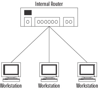
  Figure 4.12: An Internal Router

• Area border router (ABR) When a router’s interfaces are connected to different areas, that router is an ABR. An ABR has one LSDB for each area it’s connected to, as illustrated in Figure 4.13.

  
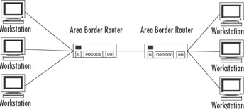
  Figure 4.13: An Area Border Router

• Backbone router If one of a router’s interfaces is on the backbone area, that router is considered a backbone router. This applies to both ABRs and internal routers.

• Autonomous system boundary router (ASBR) If a router exchanges routes with sources outside the network area, it is known as an ASBR. These special routers announce external routes throughout the area network.

Using netsh Commands

Administering your routing server through the Routing and Remote Access console is easy, but in order to pass the exam, as well as get by in the real world, you need to know how to use the command-line utility netsh, introduced in Chapter 3. You might wonder why anyone would want to use the command line when a perfectly acceptable and easy-to-use console is available. There are two main reasons:

• You can administer a routing server much more quickly from the command line. This might be especially important over slow network links.

• You can administer multiple routing servers more efficiently and consistently by creating scripts using these commands, which can then be run on many servers.

The Netsh utility is available in the Windows 2000 Resource Kit and is a standard command in Windows XP and Windows Server 2003. This utility displays and allows you to manage the configuration of your network, including both local and remote computers. It is designed to simplify the process of creating command-line scripts such as batch files. The utility itself is little more than a command interpreter that connects and interfaces with a number of services and protocols through the aid of a number of dynamic link libraries (DLLs). Each of these DLLs provides the utility with an extensive set of commands that applies specifically to that DLL’s service or protocol. These DLLs are referred to as helper files, and sometimes helper files are used to extend other helper files.

You can use the Netsh utility to perform the following tasks:

• Configure interfaces

• Configure routing protocols

• Configure filters

• Configure routes

• Configure remote access behavior for Windows 2000 and Windows Server 2003-based remote access routers that are running RRAS

• Display the configuration of a currently running router on any computer

• Use the scripting feature to run a collection of commands in batch mode against a specific router

The syntax for the Netsh utility is as follows:

netsh [-r router name] [-a AliasFile] [-c Context] [Command |      –f ScriptFile]

Context strings are appended to a command and passed to the associated helper file. The helper file can have one or more entry points that are mapped to contexts. The context can be any of the following: DHCP, ip, ipx, netbeui, ras, routing, autodhcp, dnsproxy, igmp, mib, nat, ospf, relay, rip, and wins. Under Windows XP, the available contexts include AAAA, DHCP, DIAG, IP, RAS, ROUTING, and WINS. Appending a specific context to the input string makes a whole different set of commands available that are specific to that context.

The easiest way to learn how the Netsh utility works is by viewing its help information. Open a command prompt window on your Windows Server 2003 computer and enter the netsh command at the prompt. The command prompt changes to the netsh prompt. Enter a ? to display a list of available commands, as shown in Figure 4.14. To see the subcontexts and commands that are available to use with the routing context, type routing ? at the netsh prompt (or simply type netsh routing ? at the command prompt), and then press Enter. You can get command-line help for each command by typing netsh, followed by the command, followed by ?.

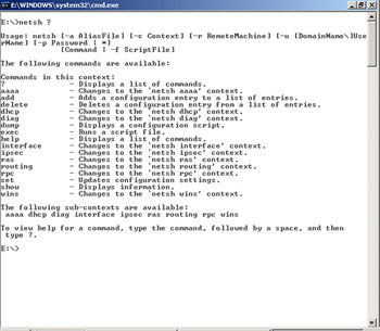
Figure 4.14: Type ? at the netsh Command Prompt to View Available Commands

Rather than entering commands through the netsh utility as shown in Figure 4.14, it is more efficient to use the DLLs without needing to load the Netsh shell. This reduces the amount of coding time required, and you can use multiple DLLs within a single script. To use Netsh commands this way, follow the netsh command with the name of the DLL and the command string. For example, to use the show helper command to see a complete list of the available DLLs, type netsh show helper, as shown in Figure 4.15.

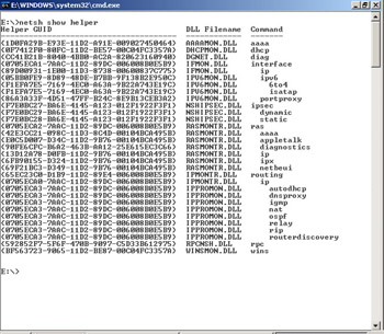
Figure 4.15: Type netsh show helper at the Command Prompt to View Available DLLs

As you can see in Figure 4.15, when the script is processed, you see the results of the script and then are returned to the command prompt, from which you can execute your next script.

Configuring & Implementing...
Using Netsh with Nested Contexts

There are times when using Netsh with simple commands is not sufficient for the tasks you want to accomplish. Sometimes, you will need to create scripts with nested contexts. Let’s take look at an example to add an interface to the network. The syntax of the command is as follows:

Add interface [InterfaceName=][InterfaceName=]InterfaceName [[IgmpPrototype=]{igmprtrv1 | igmprtrv2 | igmprtrv3 |      igmpproxy}] [[IfEnabled=]{enable | disable}] [[RobustVar=]Integer] [[GenQueryInterval=]Integer] [[GenQueryRespTime=]Integer]      [[StartUpQueryCount=]Integer] [[StartUpQueryInterval=]Integer]      [[LastMemQueryCount=]Integer] [[LastMemQueryInterval=]Integer] [[AccNonRtrAlertPkts=]{yes        | no}]

For our example, we’ll use this command to configure IGMP on a specified device. We type in the following command:

netsh routing ip igmp add interface "Local Area Connection"      startupqueryinterval = 21

This command modifies a default startup query interval to 21 seconds with IGMP configuration of the interface named Local Area Connection.

Evaluating Routing Options

EXAM 70-293 OBJECTIVE 3.1

In order to make good decisions about routing in your network, you need to evaluate potential network traffic, as well as the number and types of hardware devices and applications used in your environment. For the most part, the heavier the routing demand, the higher the need for dedicated hardware routers. Lighter routing demands can be met sufficiently by less expensive software routers. Your routing decisions should be based on your knowledge and understanding of both options.

Selecting Connectivity Devices

For small, segmented networks with relatively light traffic between subnets, a software-based routing solution such as the Windows Server 2003 RRAS might be ideal. On the other hand, a large number of network segments with a wide range of performance requirements would probably necessitate some kind of hardware-based routing solution. Evaluating your routing options includes selecting the proper connectivity devices: hubs, bridges, switches, or routers. You also should understand where these devices fit in the OSI reference model.

Head of the Class...
A Review of the OSI Model

The Open System Interconnection (OSI) reference model is an International Organization for Standardization (ISO) standard for worldwide communications. OSI defines a network framework for implementing an agreed-upon format for communicating between vendors. The model identifies and defines all the functionality required to establish, use, define, and dismantle a communication session between two network devices, no matter what the device is or who manufactured it.

All communication processes are defined in seven distinct layers with specific functionality. Microsoft and other proprietary systems may combine multiple-layer functionality into one layer in their particular version, but most, if not all, of the functionality of the original OSI model layers are incorporated. It is for this reason that most discussions of computer-to-computer communication begin with a discussion of this model. Table 4.1 shows the layers in the OSI reference model.

Table 4.1: The OSI Reference Model Layers

Layer	Description
7	Application
6	Presentation
5	Session
4	Transport
3	Network
2	Data Link
1	Physical

Layer 1 of the OSI reference model is often referred to as the bottom layer. This is the Physical layer, which is actually responsible for the transmission of the data. As a result, the Physical layer operates with only ones and zeros. It receives incoming streams of data, one bit at a time, and passes them up to the Data Link layer. Examples of transmission media associated with Layer 1 include coaxial cabling, twisted-pair wiring, and fiber-optic cabling.

Layer 2 is the Data Link layer, which is responsible for providing end-to-end validity of the data being transmitted. This layer deals with frames. The frame contains the data and local destination instructions. This means that the Physical and Data Link layers provide all the information required for communication on the local LAN. Figure 4.16 illustrates a Data Link layer domain.

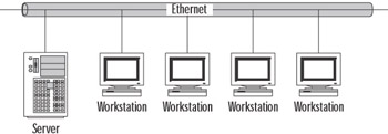
Figure 4.16: The Physical and Data Link Layers

At Layer 3, the Network layer, internetworking is enabled and the route to be used between the source and the destination is determined. There is, however, no native transmission error detection/correction method. Some manufacturers’ Data Link layer technologies support reliable delivery, but the OSI reference model does not make this assumption. For this reason, Layer 3 protocols such as IP assume that Layer 4 protocols such as TCP will provide this functionality. Figure 4.17 illustrates a network similar to the one shown in Figure 4.16, but with a second, identical network connected via a router. The router effectively isolates the two Data Link layer domains. The only way the two domains can communicate is via the use of Network layer addressing.

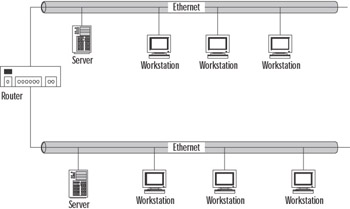
Figure 4.17: This Network Requires Network Layer Addressing

The Network layer implements a protocol that can transport data across the LAN segments or even across the Internet. These protocols are known as routable protocols because their data can be forwarded by routers beyond the local network. These protocols include IP, Novell’s Internetwork Packet Exchange (IPX), and AppleTalk. Each of these protocols has its own Layer 3 addressing architecture. IP has emerged as the dominant routable protocol. Unlike the first two layers, which are required for all applications, the use of the Network layer is required only if the two communicating systems reside on different networks or if the two communicating applications require its service.

As with the Data Link layer, the fourth layer, the Transport layer, is responsible for the end-to-end integrity of data transmissions. The main difference is that the Transport layer can provide this function beyond the local LAN. The layer detects if packets are damaged or lost in transmission and automatically requests the data to be retransmitted. This layer is also responsible for resequencing any data packets that arrived out of order.

Layer 5 of the OSI model is the Session layer. Many protocols handle the functionality of this layer in the same layer they handle the functionality of the Transport layer. Examples of Session layer services include Remote Procedure Calls (RPCs) and quality of service (QoS) protocols such as RSVP, the bandwidth reservation protocol.

Layer 6, the Presentation layer, is responsible for how the data is encoded. Not every computer uses the same data-encoding scheme. This layer is responsible for translating data between otherwise incompatible encoding schemes. This layer can also be used to provide encryption and decryption services.

Layer 7 is the Application layer. This layer provides the interface between user applications and network services.

Hubs

Hubs, sometimes referred to as repeaters, are devices used to connect communication lines in a central location and help provide common connections to all other devices on the network. A hub usually has one input and several outputs. These outputs are known as ports, but don’t confuse them with TCP/IP ports (as in port 80, the one used for HTTP traffic). These ports are just connections and nothing more. They generally accept RJ-45 connectors. Think of a hub as like the center of an old wagon wheel with all the spokes radiating out to the other part of the wheel.

A hub simply takes the data that comes into its ports and sends it out on the other ports of the hub. For this reason, it is sometimes referred to as a repeater. It doesn’t provide or perform any filtering or redirection of the data from the various sources plugged into it. Hubs are commonly used to connect various network segments of a LAN.

Hubs generally come in three flavors:

• Passive Serves simply as a pipeline allowing data to move from one device, or network segment, to another.

• Intelligent Sometimes referred to as an active, managed, or manageable hub, it includes additional features that allow you to monitor the traffic passing through the hub and configure each port for specific purposes.

• Switching Reads the destination address of each packet and forwards that packet to the correct port. Most hubs of this variety also support load balancing.

Bridges

There are several definitions for a bridge, each carrying a specific meaning when used in a particular context. In one context, a bridge can be thought of as a gateway, connecting one network to another using the same communication protocols and allowing the information to be passed from one to the other. In another context, a bridge can be used to connect two networks with dissimilar communication protocols at the Data Link layer (Layer 2), in much the same manner as a router itself. There is also a bridge called a bridge router, which supports the functions of both the bridge and the router using Layer 2 addresses for routing.

Here, we’ll look at the traditional bridge and the context that is most often associated with this device. Bridges work at both the Physical (Layer 1) and Data Link (Layer 2) layers of the OSI reference model. That means that a bridge knows nothing about protocols but forwards data depending on the destination address found in the data packet. This destination address is not an IP address, but rather a Media Access Control (MAC) address that is unique to each network adapter card. For this reason, bridges are often referred to as MAC bridges.

Basically, all bridges work by building and maintaining an address table. This table includes information such as an up-to-date listing of every MAC address on the LAN, as well as the physical bridge port connected to the segment on which that address is located.

There are three basic types of bridges:

• Transparent bridge Links together segments of the same type of LAN. A transparent bridge effectively isolates the traffic from one LAN segment from the traffic of another LAN segment, as shown in Figure 4.18.

  
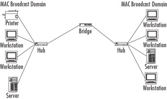
  Figure 4.18: Transparent Bridge

• Translating (or translational) bridge Like a transparent bridge, links together segments of the same type of LAN, but also can provide conversion processes needed between different LAN architectures. This allows you to connect a Token Ring LAN to an Ethernet LAN, as shown in Figure 4.19.

  
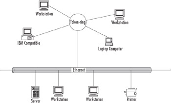
  Figure 4.19: Translating Bridge

• Speed-buffering bridge Used to connect LANs that have similar architectures but different transmission rates. Figure 4.20 shows how you might use a speed-buffering bridge to connect a 10-Mbps Ethernet network to a 100-Mbps Ethernet network.

  
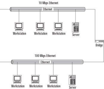
  Figure 4.20: Speed-buffering Bridge

Bridges are self-learning, so the administrative overhead is small. The functionality of bridges has been built into routers, hubs, and switches.

Switches

Switches are like bridges, except that they have multiple ports with the same type of connection (bridges generally have only two ports) and have been described as nothing more than fast bridges. Switches are used on heavily loaded networks to isolate data flow and improve the network performance. In most cases, most users get little, if any, advantage from using a switch rather than a hub.

That’s not to oversimplify and suggest that a switch doesn’t have many benefits. Switches can be used to connect both hubs and individual devices. These approaches are known as segment switching and port switching, respectively.

Segment switching implies that each port on the switch functions as its own segment. This process tends to increase the available bandwidth, while decreasing the number of devices sharing each segment’s bandwidth, but at the same time maintaining the Layer 2 connectivity. Each shared hub and the devices that are connected to it make up their own media access domain, while all devices in both domains remain part of the same MAC broadcast domain. Figure 4.21 illustrates how a segment-switched LAN can be divided to improve performance.

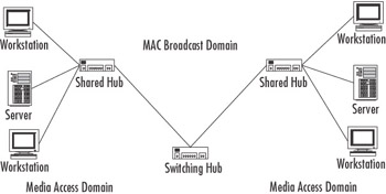
Figure 4.21: Segment Switching

Port switching implies that each port on the switching hub is directly connected to an individual device. This makes the port and the device their own self-contained media access domain. All of the devices in the network still remain part of the same MAC broadcast domain. Figure 4.22 illustrates how the media access and MAC broadcast domains are configured in a port-switched LAN.

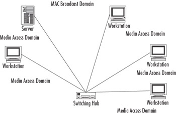
Figure 4.22: A Port-switched LAN

Layer 2 Switches

Layer 2 switches, operating at the Data Link layer, can be programmed to respond automatically to a wide range of circuit conditions. By monitoring control and data events, these switches automatically reroute circuits or switch to backup equipment, as the need requires. These switches operate using physical network, or MAC, addresses. These switches will be fast but not terribly smart. They only look at the data packet to find out where it’s headed.

Layer 3 Switches

Layer 3 switches, operating at the Network layer, are designed for disaster recovery service (or, more importantly, for disaster avoidance). These network backup units are usually designed specifically to provide high levels of automation, intelligence, and security. Layer 3 switches use routing protocols such as RIP or OSPF to calculate routes and build their own routing tables.

Layer 3 switches use network or IP addresses to identify locations on the network, identifying the network location as well as the physical device. These switches are smarter than Layer 2 switches. They incorporate routing functions to actively calculate the best way to get a packet to its destination. Unless their algorithms and processor support high speeds, though, these switches are slower.

Layer 4 Switches

Layer 4 switches, operating at the Transport layer, allow network managers to choose the best method of communicating for each switching application. Because Layer 4 coordinates communication between systems, these switches are able to identify which application protocols (HTTP, SMTP, FTP, and so forth) are included in the packets, and they use this information to hand off the packet to the appropriate higher layer software. This means that Layer 4 switches make their packet-forwarding decisions based not just on the MAC and IP addresses, but also on the application to which the packet belongs.

Because these devices allow you to set up priorities for your network traffic based on applications, you can assign a high priority for your vital in-house applications and use different forwarding rules for low-priority packets, such as generic HTTP-based traffic. Layer 4 switches can also provide security, because company protocols can be confined to only authorized switched ports or users. This feature can be reinforced using traffic filtering and forwarding features.

All these devices can be used to segment your network, but segmentation does not create separate LANs. LANs exist at only the first two layers of the OSI reference model. There’s another way to segment your network into separate LANs: use a router.

Routers

Routers are Layer 3 devices that forward data depending on the network address, not the MAC address. Since we are dealing with TCP/IP here, this means they use the IP address. Routers read the header information from each packet and determine the most efficient route by which to send that packet on its way. Think of the router as providing the link between the various networks that make up the Internet, or any other network that consists of multiple subnets. Routers isolate each LAN into separate subnets.

Like bridges, routers control bandwidth by keeping data out of subnets where it doesn’t belong. Routers, however, need to be set up before they can be used. Once they are set up, they can communicate with other routers and learn the topology of the network.

Windows Server 2003 As a Router

So, can Windows Server 2003 be used to provide routing services within your network? The answer is yes. Any computer running a member of the Windows Server 2003 family can act as a dynamic router supporting RIP, OSPF, or both. To have Windows Server 2003 provide routing services, you install multiple network interface adapters, and then enable and configure RRAS. Each network interface adapter is assigned its own IP address and subnet mask to define the directly attached network ID routes. Because you will probably use dynamic routing, default routes won’t be used, so you do not need to configure a default gateway for either network adapter.

Static IP routing will be enabled by default when the RRAS is enabled. Your next step should be to use the Routing and Remote Access administration tool to install RIP for IP or OSPF routing protocols. Next, enable the protocols on your installed network adapters by adding them to the appropriate routing protocol.

But we’re getting ahead of ourselves. Let’s start by building a checklist to follow when setting up Windows Server 2003 as a router:

• Install and configure any necessary network adapters.

• Install RRAS.

• Configure RIP or OSPF.

• Configure the remote access devices.

• Install and configure the DHCP Relay Agent.

• Install a WINS or DNS name server.

Because you’re setting up this Windows Server 2003 machine as a router, you’ll need to install two network adapters in it. You’ll also need to make sure that the necessary drivers are installed, that the TCP/IP protocol is installed, and that IP addresses have been configured on both of the network adapters. Table 4.2 shows how you might set up the IP addresses for this router.

Table 4.2: Typical Network Adapter Setup

Network Card	Connected to	IP Address
1	Backbone	192.168.0.1
2	Subnet	192.168.1.1

Your next step will be to enable RRAS on your Windows Server 2003 machine. The following exercise will walk you through this process.

Exercise 4.01: Configuring Windows Server 2003 as a Static Router

Configuring a Windows Server 2003 as a static router is simple. To follow these steps, you’ll need to be a member of the Administrators group. For security, you may want to consider using the Run As command rather than logging in with Administrator credentials.

1. If this server is a member of an Active Directory (AD) domain and you’re not a domain administrator, you’ll need to get your domain administrator to add the computer account of this server to the RAS and IAS Servers security group in the domain that this server is a member of. There’s two ways this can be accomplished.

   • Add the computer account to the RAS and IAS Servers security group using Active Directory Users and Computers.

   • Use the netsh ras add registeredserver command.

2. Select Start | Administrative Tools | Routing and Remote Access. The Welcome window appears, as shown in Figure 4.23.

   
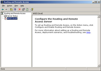
   Figure 4.23: Routing and Remote Access Welcome

3. The default is that the local computer will be listed as a server. If you want to add another server, right-click Server Status in the console tree on the left, and then click Add Server.

4. Click the appropriate option in the Add Server dialog box, as shown in Figure 4.24, and then click OK.

   
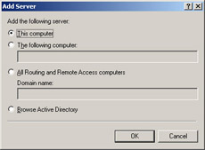
   Figure 4.24: Add a Server

5. In the console tree on the left side of the Routing and Remote Access window, right-click the server you want to enable, as shown in Figure 4.25, and then click Configure and Enable Routing and Remote Access.

   
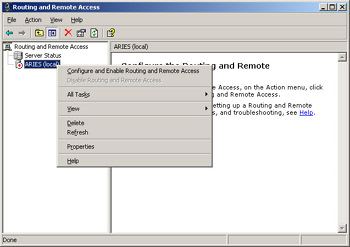
   Figure 4.25: Click Configure and Enable Routing and Remote Access

6. You’ve now started the Routing and Remote Access Server Setup Wizard, as shown in Figure 4.26. Click the Next button.

   
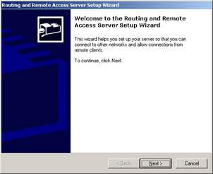
   Figure 4.26: The RRAS Setup Wizard

7. In the next window, choose the Custom configuration option, as shown in Figure 4.27. Then click the Next button.

   
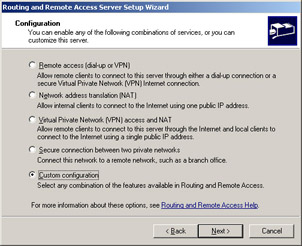
   Figure 4.27: Choose Custom Configuration

8. In the Custom Configuration window, choose LAN routing, as shown in Figure 4.28, and click the Next button.

   
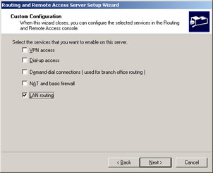
   Figure 4.28: Choose the LAN Routing Option

9. A summary of your selections will now be presented, as shown in Figure 4.29. Verify that the selections you made are correct, and then click the Finish button.

   
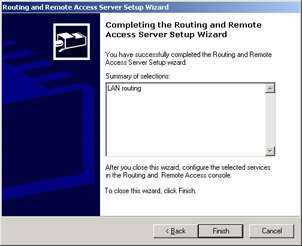
   Figure 4.29: Finish the RRAS Setup Wizard

10. A dialog box will appear, telling you that the Routing and Remote Access Service has been installed and asking you if you want to start the service, as shown in Figure 4.30. Click Yes.

    
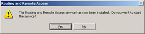
    Figure 4.30: Start the Routing and Remote Access Service

11. You should still have the Routing and Remote Access window open, and it should now look something like Figure 4.31. To add a static default route to the server, right-click Static Routes and then click New Static Route.

    
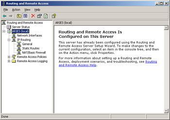
    Figure 4.31: Routing and Remote Access Window after RRAS Installation

12. Choose the interface you want to use for the default route, as shown in Figure 4.32. In the Destination text box, type 0.0.0.0. Do the same in the Network mask text box.

    
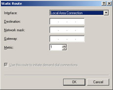
    Figure 4.32: Choose Your Interface

13. If this is a demand-dial interface, the Gateway text box will be unavailable. Select the Use this route to initiate demand-dial connections check box. This will initiate a demand-dial connection when any traffic matching this route occurs.

14. If this interface is an Ethernet or Token Ring LAN connection, in the Gateway text box, type the IP address of the interface that is on the same network segment as the LAN interface.

15. In the Metric box, type 1. Then click OK. You’ve now added a default static IP route to your router. Follow the same process (steps 11 through 15) for any other route that you want to add to the router.

After you’ve enabled RRAS, you can also add a static IP route from the command prompt using the route add command, which has the following form:

route add destination mask subnet-mask gateway metric costmetric if interface 

Where:

• Destination Specifies either an IP address or host name for the network or the host.

• Subnet-mask Specifies the subnet mask that is to be associated with this route entry. This entry defaults to 255.255.255.255.

• Gateway Specifies either an IP address or host name for the gateway or router to use when forwarding.

• Costmetric Assigns a metric cost ranging from 1 to 9,999 to use in calculating the fastest, most reliable route. This defaults to 1.

• Interface Specifies the interface you want used for the route. If you don’t specify the interface, it will be determined from the gateway IP address.

For example, to add a static route to the 192.168.1.0 network that uses a subnet mask of 255.255.255.0, a gateway of 192.168.0.1, and a cost metric of 2, type this command at the command prompt:

route add 192.168.1.0 mask 255.255.255.0 192.168.0.1 metric 2

Exercise 4.02: Configuring RIP Version 2

After you have enabled RRAS and configured a default static route, you need to enable and configure RIP on your router. This is an easy process using the Routing and Remote Access console. Follow these steps:

1. Open the Routing and Remote Access window.

2. In the console tree on the left side of the window, right-click General, and then select New Routing Protocol, as shown in Figure 4.33.

   
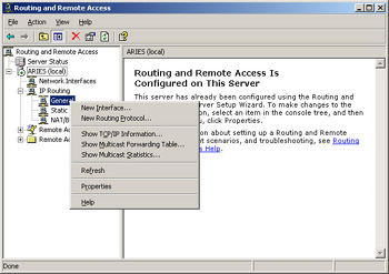
   Figure 4.33: Add a New Routing Protocol

3. From the New Routing Protocol dialog box, choose RIP Version 2 for Internet Protocol, as shown in Figure 4.34, and then click the OK button.

   
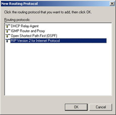
   Figure 4.34: Choose RIP Version 2 for Internet Protocol

4. RIP now appears under your server and IP Routing. Right-click RIP and choose Properties from the context menu, as shown in Figure 4.35.

   
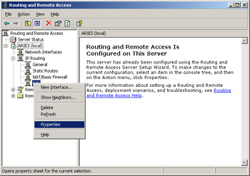
   Figure 4.35: Choose RIP Properties

5. On the General tab of the RIP Properties dialog box, shown in Figure 4.36, you can set the maximum amount of time you want this router to wait before it sends out triggered updates, as well as the level of logging you wish to have performed. Remember that triggered updates occur when the network topology changes. Updated routing information is sent out immediately reflecting that change. The General tab of the RIP Properties dialog box lets you set an interval that these triggered updates will wait before being sent. The default is five seconds. There are four levels of logging you can choose from:

   • Log errors only

   • Log errors and warnings (the default)

   • Log the maximum amount of information

   • Disable event logging

     
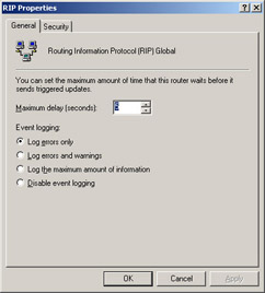
     Figure 4.36: The General Tab of the RIP Properties

     Note

     Keep in mind that logging consumes system resources so use it sparingly when you are not having network problems. When you are having a problem and you are in the process of identifying and correcting the problem, you’ll want to use the Log the maximum amount of information option, but after the problem is cleared, immediately reset logging to the default level.

6. Choose the Security tab, shown in Figure 4.37. On this tab, you can designate if this router will process announcements from routers. You can accept all announcements from all routers; you can accept announcements from the listed routers only; or you can ignore announcements from those routers listed.

   
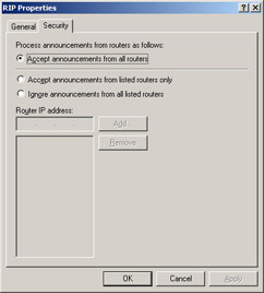
   Figure 4.37: The Security Tab of the RIP Properties

7. After you’ve made your choice, click OK.

Exercise 4.03: Configuring OSPF

You can also configure your RRAS for OSPF. Again, using the Routing and Remote Access console to configure this protocol is easy.

1. Open the Routing and Remote Access window.

2. In the console tree on the left side of the window, right-click General, as shown in Figure 4.38, and then click New Routing Protocol.

   
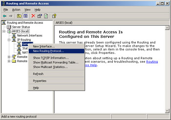
   Figure 4.38: Add a New Routing Protocol

3. In the New Routing Protocol dialog box, choose the Open Shortest Path First (OSPF) option, as shown in Figure 4.39, and then click the OK button.

   
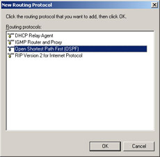
   Figure 4.39: Choose Open Shortest Path First (OSPF)

4. As with RIP, this action has now added OSPF under your server and IP Routing. Right-click OSPF and choose Properties.

5. You’re offered similar choices to those that are available when you configure RIP (see Exercise 4.2). After you’ve made your choices, click OK.