Chapter 49: Modeling Nonlinearities and Interactions | MicrosoftВ® Office ExcelВ® 2007: Data Analysis and Business Modeling (Bpg -- Other)

Overview

What does it mean when we say that an independent variable has a nonlinear effect on a dependent variable?
What does it mean when we say that the effects of two independent variables on a dependent variable interact?
How can I test for the presence of nonlinearity and interaction in a regression?

What does it mean when we say that an independent variable has a nonlinear effect on a dependent variable?
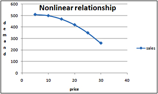
An independent variable will often influence a dependent variable through a nonlinear relationship. For example, if we try to predict product sales using an equation such as Sales=500–10*Price, price influences sales linearly. This equation indicates that a unit increase in price will (at any price level) reduce sales by 10 units. If the relationship between sales and price were governed by an equation such as Sales=500+4*Price– .40*Price², price and sales would be related nonlinearly. As shown in Figure 49-1, larger increases in price result in larger decreases in demand. In short, if the change in the dependent variable caused by a unit change in the independent variable is not constant, there is a nonlinear relationship between the independent and dependent variables.

Figure 49-1: Nonlinear relationship between demand and price
What does it mean when we say that the effects of two independent variables on a dependent variable interact?
If the effect of one independent variable on a dependent variable depends on the value of another independent variable, we say that the two independent variables exhibit interaction. For example, suppose we try to predict sales using price and the amount spent on advertising. If the effect of changing the level of advertising dollars is large when the price is small and small when the price is high, price and advertising exhibit interaction. If the effect of changing the level of advertising dollars is the same for any price level, sales and price do not exhibit any interaction.
How can I test for the presence of nonlinearity and interaction in a regression?
To see whether an independent variable has a nonlinear effect on a dependent variable, we simply add an independent variable to the regression that equals the square of the independent variable. If the squared term has a low p-value (less than 0.15), we have evidence of a nonlinear relationship.
To check whether two independent variables exhibit interaction, we simply add a term to the regression that equals the product of the independent variables. If the term has a low p-value (less than 0.15), we have evidence of interaction.
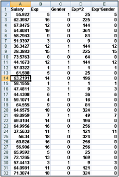
To illustrate, let’s try to determine how gender and experience influence salaries at a small manufacturing company. For each employee, we are given the following set of data. You can find the information in the Data worksheet in the file Interactions.xlsx, shown in Figure 49-2.

Figure 49-2: Data for predicting salary based on gender and experience
- Annual salary (in thousands of dollars)
- Years of experience working in the manufacturing business
- Gender (1=female, 0=male)
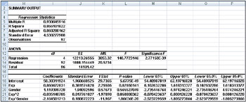
We’ll use this data to predict salary (the dependent variable) based on years of experience and gender. To test whether years of experience has a nonlinear effect on salary, I added the term Experience Squared by copying from D2 to D3:D98 the formula B2^2. To test whether experience and gender have a significant interaction, I added the term Experience*Gender by copying from E2 to E3:E98 the formula B2*C2. I ran a regression with an Input Y Range of A1:A98 and an Input X Range of B1:E98. After checking the Labels box in the Regression dialog box and clicking OK, I got the results shown in Figure 49-3.

Figure 49-3: Regression results that test for nonlinearity and interaction
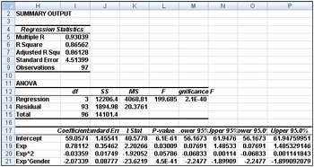
We find that gender is insignificant (its p-value is greater than 0.15). All other independent variables are significant (meaning they have a p-value less than or equal to 0.15). We can delete the insignificant gender variable as an independent variable. To do this, I copied the data into a new worksheet called FinalRegression (right-click any worksheet tab, click Move Or Copy, and check the Create A Copy box.) After deleting the Gender column, we obtain the regression results included in the FinalRegression worksheet and shown in Figure 49-4 on the next page.

Figure 49-4: Regression results after deleting insignificant gender variable
All independent variables are now significant (have a p-value less than or equal to 0.15). Therefore, we can predict salary (in thousands of dollars) by using the following equation (equation 1):
```
 Predicted salary=59.06+.78(EXP)-.033EXP²⁻2.07(EXP*GENDER)
```
The negative EXP² term indicates that each additional year of experience has less impact on salary, which means that experience has a nonlinear effect on salary. In fact, our model shows that after 13 years of experience, each additional year of experience actually reduces salary.
Remember that gender equals 1 for a woman and 0 for a man. After substituting 1 for gender in equation 1, we find that for a woman:
```
 Predicted salary=59.06+78EXP-.03EXP²⁻2.07(EXP*1)=59.06-.033EXP2 − 1.29EXP
```

For a man (substituting gender=0), we find that:

 Predicted salary=59.06+.78EXP-.03EXP²⁻2.07(EXP*0)=59.06+.78EXP-.033EXP²

Thus, the interaction between gender and experience shows that each additional year of experience benefits a woman an average of 0.78–(–1.29)=$2,070 less than a man. This indicates that women are not being treated fairly.