13.2. Descriptive Names for Cell References One of the obvious problems with Excel formulas is that they don't make for the easiest reading in the world. Consider this formula: =(A1+A2)*B1
It's immediately obvious that this formula adds together two numbers (the numbers in cells A1 and A2), and multiplies the result by a third number (the number in cell B1). However, the formula gives absolutely no clue about the purpose of this calculation. There's no way to know whether it's converting currencies, calculating a discount, or measuring the square footage of your llama day care center. To answer these questions, you need to look at the worksheet and track down the cells this formula references. On the other hand, consider the next formula, which uses descriptive names in place of cryptic cell references. Although it performs the same calculation, this formula provides much more information about what it's actually trying to accomplishcalculating the retail price of a product: =(ProductCost + ShippingCost) * MarkupPercentage
Excel lets you build formulas using such descriptive names, or named ranges . All you have to do is define the ranges as you create your worksheet, and then you can use these names instead of cell references. Named ranges provide other benefits besides conveying the meaning of a formula: -
They make complex, nested formulas more understandable. -
They make it easy to quickly find a cell or select a group of cells. That makes them ideal for navigating large worksheets or for applying formatting to cell ranges that frequently change. -
They reduce the likelihood of some types of errors. For example, you're unlikely to notice if you've used A42 instead of A41, but you can spot the wrong name when you use TotalWithTax instead of TaxRate. -
They use absolute references. That way, you don't need to worry about having a formula change when you copy a formula from one cell to another. (Although 99.9 percent of all Excel fans use absolute references for named ranges, this Excel rule is one you can break for some unusual tricks. To learn about this technique and other unusual tricks, check out Excel 2007 Hacks by David and Raina Hawley [O'Reilly].) -
They add an extra layer between your formulas and your worksheet. If you change the structure of your worksheet, then you don't need to modify your formulas. Instead, you simply need to edit the named ranges so they point to the new cell locations. This ability is particularly useful when writing macros (Chapter 27) because it lets you avoid writing direct cell references into your code. In the next few sections, you'll learn how to create named ranges. You'll also pick up a few tricks for defining and applying names automatically. 13.2.1. Creating and Using a Named Range Creating a named range is easy. Just follow these steps: -
Select the cells you want to name . You can name a single cell or an entire range of cells. -
Look for the box at the left end of the formula bar, which indicates the address of the current cell (for example, C5). This part of the formula bar is called the name box . Click the name box once . The text inside (the cell address) is now selected. -
Start typing the name you want to use . What you type replaces the cell address (see Figure 13-4). 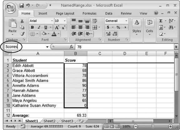 | Figure 13-4. This worksheet has a named range so you can easily use the student grades in your formulas without remembering specifically where the cells are. (It also lets you change the range and update all your formulas in one step, if the worksheet changes.) To define the range for student scores, simply select the cells with the numeric scores (B2 to B10), and then enter the new name using the name box in the formula bar (circled). | | -
Press Enter to confirm the new name . You can now select the name at any time (see Figure 13-5). To use a name, click the drop-down arrow to the right side of the name box to show a list of all the names that are defined in the workbook. When you click a name, Excel jumps to the appropriate position and selects the corresponding cell or range of cells.
Note: When you name a range, you have to follow certain rules. All names must start with a letter, and they can't contain spaces or special charactersexcept the underscore ( _ ). Also, all names must be unique. Finally, you can't create a range name that matches a valid cell address. For example, BB10 isn't a valid range name because every worksheet has a cell with the address BB10.
Once you've created a name, you can use the name in any formula, just as you would any cell reference or cell range. As a shortcut, you can pick the name from a handy list. To do so, start entering your formula, and then select Formulas  Defined Names Use in Formula. This selection pops open a menu with all the names youve defined in your workbook. Select the name you want to use, and then Excel inserts it into the formula. Defined Names Use in Formula. This selection pops open a menu with all the names youve defined in your workbook. Select the name you want to use, and then Excel inserts it into the formula. 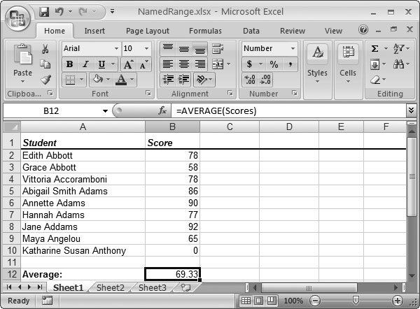 | Figure 13-5. Once you've defined and named a cell range, you can use it in two ways: in existing formulas (as demonstrated with the AVERAGE() function here), or you can select the name from the formula bar's drop-down list (which automatically selects the cells in the range). | |
13.2.2. Creating Slightly Smarter Named Ranges The name box gives you a quick way to define a name. However, you have other ways to supply a few optional pieces of name- related information, like a description. To create a name with this optional information: -
Select the cells you want to name . -
Choose Formulas Defined Names Define Name . Or, without using the ribbon, just right-click the selected cells, and then choose Name a Range. Either way, the New Name dialog box appears (Figure 13-6). 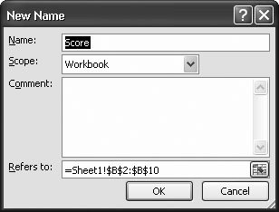 | Figure 13-6. In the New Name dialog box, you fill in the standard name and cell reference information, along with two extra details: the ever-important Scope setting (which lets you organize names in workbooks with multiple worksheets) and a Comment setting (which lets you add descriptive text that explains your name). | | -
Fill in the information for your named range . The only information you need to add is the name, but you can tweak several settings: -
Name is the name you're giving to the range (like TaxRate). -
Scope lets you control where you're allowed to use the name. Ordinarily, names have Workbook scope, which means you can use them on any worksheet in your workbook. However, you may choose to limit the scope to a single, specific worksheet instead. This way, your name lists aren't as cluttered, because you see only the names for the current worksheet. Also, you don't need to worry about using the same name in different worksheets. Worksheet-scoped names are almost always the best way to go. -
Comment is a description for your named range. This description appears in a tooltip when you enter the name into a formula. You can use any text you want for the comment, but Excel experts use it to describe what type of information's in the cells, when the data was last updated, and whether the range depends on information in other workbooks. -
Refers to is a cell reference that indicates the cells you selected in step 1. If you didn't get it quite right, then you can modify the range now. -
Click OK to create the name . You can now use your name in formulas anywhere . In fact, Excel even helps you out with its Formula AutoComplete feature, as shown in Figure 13-7. 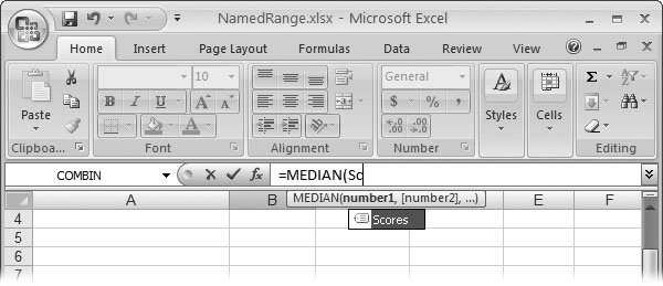 | Figure 13-7. Excel's AutoComplete feature doesn't just suggest possible function namesit also shows you the named ranges that match the text you've typed so far. And if your name has a comment, you see that text appear in a tooltip to help you out. | |
13.2.3. Naming Formulas and Constants The New Name dialog box also provides the key to unlock additional naming features. Using this dialog box, you can create names that point to things other than cell ranges. You can create nicknames for frequently used formulas (such as "My_ Net_Worth"). This section describes how. Internally, Excel treats all names as formulas. That is, when you create a named range, Excel simply generates a formula that points to that range, like = $A$1: $A$10 . To check this out, select a few cells, and then choose Formulas Defined Names Define Name. In the "Refers to text box at the bottom of the window, you see a formula with the corresponding cell reference. Although most names refer to cell ranges, there's no reason why you can't create names with different formulas. You can use this approach to define a fixed constant value that you want to use in several formulas. Here's an example: =4.35%
To create this constant, enter the name in the text box at the top of the New Name dialog box (for example, SalesCommission), enter the formula in the "Refers to" text box, click Add, and then click OK. You can now use this name in place of the constant in your worksheet calculations: =A10*SalesComission
People often use named constants to make it easier to insert frequently used text. You may want to declare a company name constant: ="Acme Enterprises, Incorporated."
You can then use that text in a number of different cells. And best of all, if the company name changes, you simply need to update the named formula, no matter how many times it occurs on the worksheet! Similarly, you can create names that reference more complex formulas. These formulas can even use a combination of functions. Here's an example that automatically displays the name of the current day: =TEXT(TODAY(), "dddd")
Tip: Overall, you'll probably find that the most useful type of name is one that refers to a range of cells. However, don't hesitate to use named constants and named formulas, which are particularly useful if you have static text or numbers that you need to use in multiple places.
13.2.4. Managing Named Ranges It's all well and good to create named ranges, but sooner or later you'll need to tweak your handiwork by doing things like deleting names you don't need anymore, or editing the ones you regularly use (so that they designate a different area, for example). For these tasks , you need to choose Formulas Defined Names Name Manager to show the Name Manager (as shown in Figure 13-8). The Name Manager is the starting point when you need to add, delete, or edit existing named ranges. Here's what you can do: -
To add a name , click New. You get to the familiar New Name dialog box. 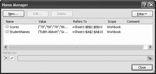 | Figure 13-8. The Name Manager shows you a list of all the names in your workbook. For better organization, you can click a column to re- sort the list. You can also resize the window to see more names at once. | |
-
To remove a name , select it in the list, and then click Delete. Any formulas using that name display the error code #NAME? or #REF! , indicating that Excel can't find the named range. -
To edit a name , select it in the list, and then click Edit. You see an Edit Name dialog box, which looks exactly the same as the New Name dialog box. Excel's nice enough to keep track of names. If you rename TaxRate to TaxPercentage, Excel adjusts every formula that uses TaxRate so it uses TaxPercentage, thereby avoiding an error.
Tip: If you need to change the cell reference for an existing name, but you don't need to change anything else (like its name or comment), Excel's got a quicker way. Just select the name in the list, and then modify the cell reference in the "Refers to" box at the bottom of the window. (Click-lovers can change the cell reference using the mouse. Just click inside the "Refers to" box so the cell reference becomes highlighted on the worksheet. Then, drag on the worksheet to draw the new cell reference.)
The Name Manager is a great place to review all the names you're using, check for errors, and make adjustments. Many Excel experts create workbooks that have hundreds of names. If you find yourself in this situation, then you may have a hard time finding the names you want in the list of names. Fortunately, the Name Manager includes a filtering feature that can help. Filtering cuts down the name list so that instead of showing all the names in your workbook, it shows only the names you're interested in. The Name Manager lets you use several types of filters: -
You can find names that are limited to the current worksheet. -
You can find names that point to cells with errors (and those that don't). -
You can find ordinary names, or names used in tables (Chapter 14). Figure 13-9 shows the filter settings you can choose from. 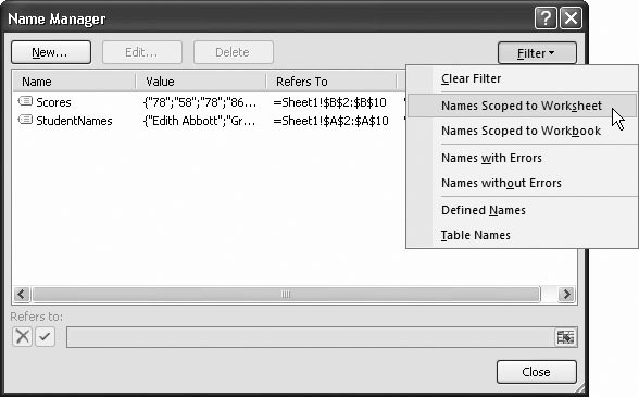 | Figure 13-9. To apply a filter, click the filter button, and then make a choice from the drop-down menu. You'll notice that this menu has several sections, separated by horizontal lines. Each section represents a separate type of filter. If you want, you can apply a filter from more than one section at once. You can look for names that are limited to the current worksheet and point to cells with errors, as in this example. To get back to normal and show all names, choose Clear Filter. | |
GEM IN THE ROUGH
Getting a List of Names | | After defining dozens of different names on a worksheet, you may appreciate an easy way to review them. The Name Manager is a great tool while you're using Excel, but there's another choice that lets you look over your names from the comfort of your armchair. You can paste a list of all your names into a worksheet, complete with their cell references. (Typically, you don't keep this list in your worksheet. Instead, you create it, print it out, and then remove it.) To generate the list of names, click the cell where you want to start the list. Remember, you need two free columnsone for the range names and one for the range addressesand you don't want to overwrite any existing data. Once you're at the right place, select Formulas Defined Names Use in Formula Paste Names. When the Paste Name dialog box appears, click the Paste List button. This name list is static, which means Excel doesn't update it if you add more names to your worksheet. Instead, you need to generate the list again. |
13.2.5. Automatically Creating Named Ranges Excel also has the built-in smarts to automatically generate named ranges for you. To perform this trick, Excel searches a group of cells you select and, with a little help from you, identifies which cell or cells would serve as appropriate names. If you have a column title in cell A1, Excel can use the text in that cell to label the range of cells underneath it. To use automatic naming, follow these steps: -
Select the cells for which you want Excel to create one or more named ranges . Excel lets you quickly create one or more named ranges. Your selection must include the cells that you want to be part of the named range, plus the cell or cells that contain the descriptive text. Figures 13-10 and 13-11 show examples. 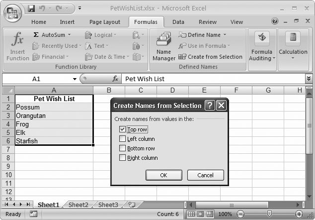 | Figure 13-10. Excel helps you quickly create named ranges. Use the "Create Names from Selection" dialog box to indicate which cells Excel should use to generate the names. If you just want to create a single named range (from a vertical list, for example), then you'd pick Top Row in the Create Names dialog box. Here, the named range is Pet_Wish_List (Excel automatically inserts underscores in place of spaces), and the included cells in this range are A2 to A6. | | 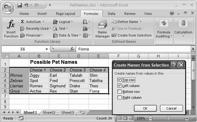 | Figure 13-11. You can also use "Create Names from Selection" with a table of data. In this case, by turning on Left Column, Excel uses each of the animals in column A as the title for a different named range. The Rhinos range, for example, contains cells B3 to E3. If you turn on the Top Row checkbox, then Excel also creates named ranges for each column, like Choice_1 (cells B3:B6), Choice_2 (cells C3:C6), and so on. It's up to you whether you want to create ranges for row headings, column headings, or both. | | -
Choose Formulas Defined Names Create from Selection . The "Create Names from Selection" dialog box appears. -
Specify which part of your selection has the text label (or labels) you want to use by turning on the appropriate checkbox . In order to create a name, Excel has to find some text to use as a label. You use the Create Names dialog box to tell Excel where that text is. If the text is contained in column headings, then select "Top row." If there are row and column headings, then select "Top row" and "Left column." Excel selects the options that it thinks make sense based on your selection. -
Click OK to generate the names . Excel's automatic naming ability seems like a real timesaver, but it can introduce as many problems as it solves . Here are some of the quirks and annoyances to watch out for: -
The named ranges may not be the ones you want, especially if you use long, descriptive column titles. The name Length is more manageable than the name Length_in_Feet which is what Excel sticks you with if your name-containing cell happens to contain the text Length in Feet . You could rename your named range after the fact (Section 13.2.4), but it's extra work. -
If you frequently use the Create Names tool, you may suddenly find yourself with dozens of names, depending on your worksheet's complexity. Since you haven't created these names yourself, you won't necessarily know what each one references. One way to figure it out is to use the technique described in the box in Section 13.2.5. -
Excel doesn't generate names if your column or row labels contain only numbers. If you have a table with a list of part numbers or customer IDs, then Excel assumes the numbers are a part of the data, and not labels it can use for naming. And if your column or row names are text values that start with a number (like "401K"), then Excel adds an underscore at the beginning to make a valid name ("_401K"). -
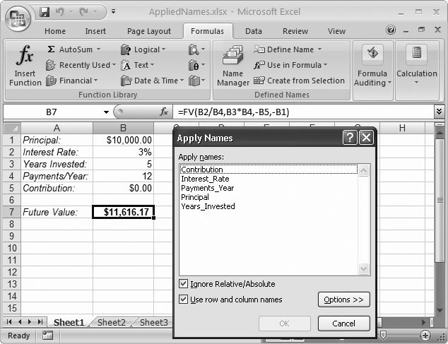
If you don't have any row or column labels, Excel can't generate any names. 13.2.6. Applying Names to Existing Formulas Named ranges are extremely helpful, but unless you've planned out your spreadsheet writing in a careful, orderly manner, you may find that you spend more time managing these names than actually using them. Suppose you've written a bunch of formulas that work their magic on a table of data that doesn't use any named ranges. Then, after you've written the formulas, you catch the named range bug and apply names to, say, all the columns in your table. Your formulas still work, but they don't use the names you've just created.
Note: There's one thing to remember before you get started with the Apply Names feature. Excel can use named ranges only if you've defined them. If your worksheet doesn't include any named ranges, or if they don't match the ranges used in your formulas, this feature doesn't do anything.
So you've either got to go through and manually revise each formulaso that, for example, = SUM(A2:A85) becomes = SUM(My_Stocks) or, if you're not a fan of carpal tunnel syndrome, you can use one of Excel's most valuable shortcuts: the ability to automatically replace old-school alphanumeric cell references with reader-friendly named range labels. To use this time-saving technique, follow these steps: -
Select the cells that contain the formulas you want to change . Of course, you'll want to use this shortcut only if you've got a bunch of formulas that don't yet use one or more existing named ranges. Select the cells that contain the formulas you want to change. This shortcut can work on more than one formula at a time (even if each formula references a different named range), so it's OK to select a group of formulas. -
Select Formulas Defined Names Define Name Apply Names . The Apply Names dialog box appears (Figure 13-12), with a list of all the names in your workbook. Excel searches for and highlights the appropriate names. If your formulas have ranges you don't want to use, then deselect them. If the Ignore Relative/Absolute checkbox is turned on, Excel changes any matching reference, whether it's absolute or relative. This behavior's usually what you want because most people writing formulas use relative references (like A2 instead of $A$2)unless they explicitly need absolute references to make copying and pasting easier. If you don't turn this option on, then Excel replaces only absolute references. You'll also notice the "Use row and column names" checkbox. This setting applies only if you generated names using the Formulas Named Cells Create from Selection technique described in the previous section. If youve used this technique to create row and column names, then you can turn off the "Use row and column names" checkbox to prevent Excel from using these names in your formulas. You may skip this step because Excel can create horribly complex formulas with the row and column names. That's because in order to get a specific cell in a range, Excel uses range intersection . Consider the grid of pet names in Figure 13-11. If you apply names with the "Use row and column names" checkbox turned on, then Excel converts a simple formula like = B3 into = RHINOS Choice_1 . In other words, Excel notices that the intersection of the RHINOS range (B3:E3) and the Choice_1 range (B3:B6) is the single cell B3. You may consider this either an elegant adjustment or an unnecessary way to complicate your life. -
Click OK to apply the names . Every time Excel finds a range that matches one of the highlighted range names, it replaces the alphanumeric cell reference with the range name. |