Section 13.1. Conditions in Formulas | Excel 2007[c] The Missing Manual

13.1. Conditions in Formulas

Chapter 8 gave you a first look at how to use conditional logic when writing Excel formulas. The basic principles are easy: you construct a condition using the logical operators like <, >, =, and <>, and then use this condition with a conditional function . So far, you've considered only one conditional functionIF()which performs different actions depending on the result of a calculation.

The following formula carries out the operation in either the second or third argument, depending on the value of cell A20:

 =IF(A20>10000, A20*5%, A20*3%)

Translation: For values greater than 10,000, Excel executes the formula A20*5% ; otherwise , it carries out the second formula. If A20 contains the dollar amount of a sales invoice, you can use this formula to determine the commission for a sales person. If the sale exceeds the magic $10,000 amount, a larger five percent commission kicks in.

13.1.1. IF(): Building Conditional Formulas

IF() is one of the most useful conditional functions, but it's not the only one. In fact, you'll find several more logical functions in the Formulas Function Library Logical category. These formulas include the IFERROR() function you tackled in Section 12.3.1, and the following:

TRUE() and FALSE() . These functions don't take any arguments. The TRUE() function simply returns the logical value true , and the FALSE() function returns false . You can use these functions to enter logical values directly into a cell or formula, but you won't need them very often.
AND() . This function accepts two (or more) conditions, and then returns true if all of them are true. If any condition's false, the AND() function returns false .
OR() . This function accepts two (or more) conditions, and then returns true if any one of them is true. The OR() function returns false only if all conditions are false.
NOT() . This function accepts a condition and reverses it. Consider the formula = NOT(ISBLANK(A10)) . Assuming A10 is empty, the ISBLANK() function returns true; by contrast, the NOT() formula returns the reverse false . You rarely need the NOT() function, but sometimes it helps make your logic a little clearer.

On their own, these logical functions don't accomplish much. However, you can combine them in some interesting ways with the IF() function. Imagine you want to make sure the 5 percent rate (from the sales commission example) kicks in only if the sale exceeds $10,000 and the sale occurs after the year 2006, when the new commission rules came into effect. You can rewrite the earlier formula to take this fact into account using the AND() function. If the invoice date's in cell B4, here's what the formula would look like:

 =IF(AND(A20>10000,YEAR(B4)>2006), A20*5%, A20*3%)

Similarly, you may encounter a situation where you want to alter your logic so that the higher commission rate kicks in if at least one of two different criteria is met. In this case, you'd use the OR() function.

Tip: The information functions described in Chapter 12 are also quite useful in conditional statements. The "IS" functions, like ISERROR() and ISBLANK(), especially lend themselves to these statements.

You can also choose between more than two options by nesting multiple IF() statements in a single formula. (Nesting is a technique that lets you put one function inside another.) The following formula uses a commission of two percent if the sale is under $500, a commission of five percent if the total is above $10,000, and a three percent commission for all other cases.

 =IF(A20<500, A20*2%, IF(A20>10000, A20*5%, A20*3%))

The formula begins by checking the first condition (whether A20 is less than $500). If the condition is met, then Excel carries out the first expression, A20*2% . If A20 is not less than $500, Excel moves on to the second expression, which is actually another IF() function. It then checks the second condition and chooses between the two remaining commission levels.

Excel allows up to a staggering 64 nested IF() statements in one formula. (This limitation actually applies to all Excel functions. You can't nest functions more than 64 levels deep.) However, it's unlikely that anyone could actually understand a formula with 64 IF() statements. Nesting IF() statements may get the job done, but it can lead to some extremely complicated formulas, so tread carefully .

Note: In some situations, nesting multiple IF() statements may cause the formula to become too complex and error-prone . In these cases, you may want to consider simplifying your logic by breaking it into several linked formulas, or building a custom function using full-fledged VBA (Visual Basic for Applications) code. You'll see an example of that in Chapter 28.

Along with the functions in the Logical category, Excel also includes a few more functions that use conditions. These functions include the COUNTIF() and SUMIF() functions, as described in the next two sections.

13.1.2. COUNTIF(): Counting Only the Cells You Specify

To understand the purpose of COUNTIF() and SUMIF(), you need to remember that the COUNT() and SUM() functions devour everything in their path . But what if you want to pick out specific cells in a range and count or sum only these cells? You might try to use COUNT() or SUM() in conjunction with an IF() statement, but that doesn't solve the problem. Consider the following formula:

 =IF(ISBLANK(A1), 0, COUNT(A1:A10))

This formula checks to see if cell A1 is blank. If it's blank, the formula returns 0. If it isn't blank, the formula returns the count of all the numeric values from A1 to A10. As you can see, the actual counting operation's an all-or-nothing affair. Excel either counts all of the cells or ignores them all. There's no way to count just some of the cells (or, similarly, add just some of the cells). The COUNTIF() and SUMIF() functions address this issue by letting you specify a condition for each cell .

The COUNTIF() function is the more straightforward of the two. It takes two parameters: the range of cells you want to count, and the criteria that a cell needs to satisfy in order to be counted:

 COUNTIF(range, criteria)

The criteria argument is the key to unlocking the real power of COUNTIF(). The formula tests every cell in your range to see if it meets your criteria, and counts only if it does. With the criteria you can:

Test if a cell matches a specific value.
Test if a cell is greater or less than a specific number.
Test if a cell matches, or is greater or less than, a number in another cell.
Test if a cell contains text that matches a simple pattern.

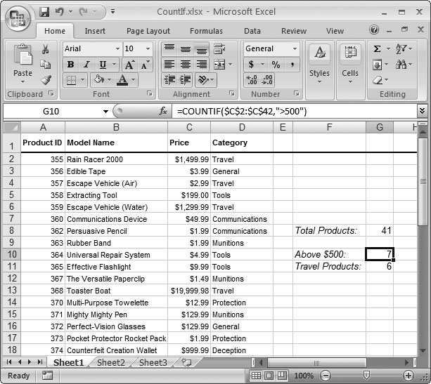
Consider the list of products shown in Figure 13-1, which stretches from row 2 to 42. Counting the number of products is easyyou just use the plain- vanilla count function:

 =COUNT(A2:A42)

This formula returns 41 , which is the total number of non-blank cells in the range. Now, what if you want to count how many products are priced over $500? This challenge calls for the COUNTIF() function. Here's the formula:

Figure 13-1. This worksheet shows a list of products. The COUNT() function makes it easy to count the products, but COUNTIF() gives you the additional ability to count only those products that reach a set price threshold or are in a certain category.

 =COUNTIF(C2:C42, ">500")

Note that, in this case, the formula counts the cells in column C. That's because column C contains the price information for each product, which you need in order to evaluate the condition. (When using the COUNTIF() function, the condition in the second argument's always a string, which means you need to make sure to place it inside quotation marks.)

To understand how the criteria argument works, you need to realize that it's not a logical condition like the ones used with the IF() statement. Instead, it's a snippet of text that contains part of a condition. When COUNTIF() springs into action, it creates a full condition for each cell in its assigned range. In the formula shown earlier, the criteria is > 500 . Each time the COUNTIF() function tests a cell, it uses this criteria to generate a full-fledged condition on the fly. The first cell in the range is C2, so the condition becomes C2 > 500 . If the condition is true (and for C2, in Figure 13-1, it is), COUNTIF() counts the cell.

Using this logic, you can easily construct other conditional counting formulas. Here's how you'd count all the products in the Travel category (column D) by examining the cells in the Category column:

 =COUNTIF(D2:D42, "=Travel")

Tip: If your condition uses the equal sign, you can omit it. For example, COUNTIF() assumes that the condition "Travel" is equivalent to "=Travel" .

UNDER THE HOOD
How Excel Compares Different Types of Data

The type of data that's in a cellordinary numbers, text, or datesinfluences how Excel compares it in a condition. If you use the greater than (>) and less than (<) symbols with numbers , Excel performs the expected numeric comparison. However, if you use these symbols with text, Excel performs a letter-by-letter alphabetic comparison, which means Excel considers the word apple less than banana because the first letter, a, occurs before b in the alphabet. Comparisons are always case-insensitive, so tRaVeL matches Travel .

Date and time comparisons work the same as numeric comparisons, although it helps to remember that Excel stores dates as a number of days (see Section 2.2 for an explanation) and times as a fractional number between 0 and 1. In other words, Excel deems that dates or times in the past are smaller than more recent dates in a comparison.

Finally, Excel lets you use the asterisk (*) wildcard when you're making text comparisons. The asterisk stands for any sequence of characters . Thus, the criteria "=T*" matches any cell that contains text that starts with the letter T. Here's how you'd use it with the COUNTIF() function:

 =COUNTIF(D2:D42,"=T*")

This formula matches any category that starts with the letter T, which includes Travel and Tools.

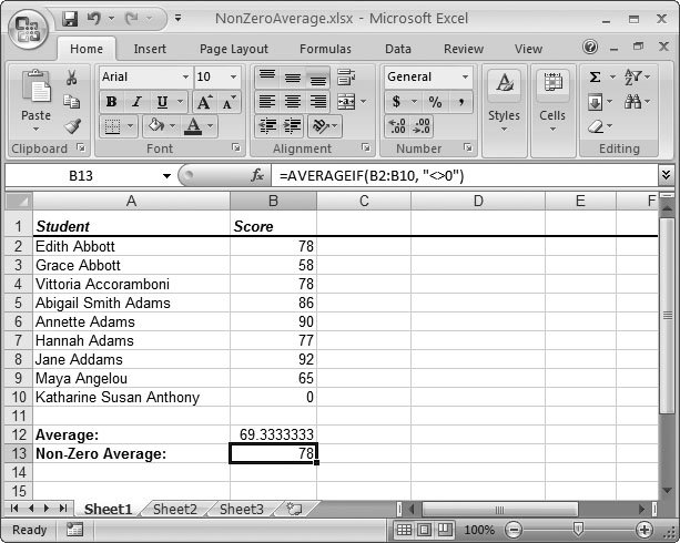
You can even draw the information you want to use in your condition from another cell. In this case, you simply need to use the text concatenation operator (&) to join together the cell value with the conditional operator you want to use. (See Section 11.1 for an explanation of how concatenation works.) If the reader of your spreadsheet enters the category name in cell G1, you could count matching products using the following formula:

 =COUNTIF(D2:D42, "=" & G1)

This formula joins the equal sign to whatever text is in cell G1. Thus, if G1 has the text Tools, the criteria becomes "=Tools" .

You can use a similar technique to use a function in the criteria argument. Here's a formula that counts the number of products that are above the average price:

 =COUNTIF(C2:C42, ">" & AVERAGE(C2:C42))

13.1.3. SUMIF(): Adding Only the Cells You Specify

The SUMIF() function follows the same principle as COUNTIF(). The only difference is that it accepts an optional third argument:

 SUMIF(test_range, criteria, [sum_range])

The first argument is the range of cells you want the criteria to test, the second is the criteria itself, and the third is the range of cells you want to sum. So if the first cell in test_range passes the test (that is, causes the criteria to evaluate to true ), the function adds whatever the first cell is in the sum_range to the total sum. Both test_ range and sum_range must have the same number of cellsusually they'll be different columns in the same table.

Imagine you want to calculate the sum of all the products in the Travel category, as shown in Figure 13-1. In this case, you'd want to test the cells from the Category column (D2:D42) to see whether they contain the word Travel; these cells comprise your test range. But then you would want to add the cells from the Price column (C2:C42), and those cells would be your sum range. Here's the formula:

 =SUMIF(D2:D42, "=Travel", C2:C42)

The two ranges (D2:D42 and C2:C42 in this example) need to have the same number of cells. For each cell Excel tests, that's one cell it may or may not add to the total.

If you omit the sum_range argument, the SUMIF() function uses the same range for testing and for summing. You could use this approach to calculate the total value of all products with a price above $500:

 =SUMIF(C2:C42, ">500")

For many generations of Excel, enterprising spreadsheet writers were limited to SUMIF() and COUNTIF(). In Excel 2007, one more IF-formula appears: AVERAGEIF(), which calculates the average of cells that fit set criteria. Figure 13-2 shows an example.

Figure 13-2. Here are two approaches to calculate an average. The formula in B13 ignores all scores of 0, which represent students who didn't take the test. The result of 78 percent (returned by the AVERAGEIF() function) is clearly quite a bit higher than the value of 69 percent and change (returned by the AVERAGE() function), but it's a more realistic representation of student performance.

13.1.4. COUNTIFS() and SUMIFS(): Counting and Summing Using Multiple Criteria

The COUNTIF(), SUMIF(), and AVERAGEIF() functions suffer from one limitation: They can evaluate cells using only one criteria. In the past, spreadsheet creators have been forced to use some creative thinking to work around this problem. (Possible solutions include using an array formula or relying on the cryptic SUMPRODUCT() function, which multiplies two ranges together.) Fortunately, this sleight-of-hand isn't required in Excel 2007 because several new functions solve the problem:

SUMIFS() is the same as SUMIF(), except it accepts multiple conditions.
COUNTIFS() is the same as COUNTIF(), except it accepts multiple conditions.
AVERAGEIFS() is the same as AVERAGEIF(), except it accepts multiple conditions.

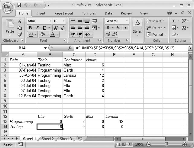
If you're truly demanding, you'll be happy to know that all three of these functions accept over 100 separate conditions.

Earlier in this chapter you saw how you could use COUNTIF() either to count the number of products over $500 or to count the number of travel products in the list. But what if you want to use both conditions at oncein other words, you want to zero in on just those travel products that pass the $500 threshold? In this situation, you need COUNTIFS() to evaluate your two conditions. The following explanation builds the formula you need one piece at a time. (See Figure 13-1 if you need help visualizing the spreadsheet that this formula is searching.)

The first argument for COUNTIFS() identifies the range you want to use to evaluate your first condition. In this example, this first condition tests whether a product's in the Travel category. In order to test this condition, you need to grab the entire Category column, like so:

 =COUNTIFS(  D2:D42,  )

Now, you need to fill in the condition that Excel uses to test each value. In this case, you need a condition that checks that the value matches the text "Travel":

 =COUNTIFS(D2:D42,  "=Travel",  )

The fun doesn't stop here. You can use the same technique to fill in the second condition, which looks for prices that exceed $500 dollars. Once again, you fill in the range you want to use (this time it's the Price column) and the condition:

 =COUNTIFS(D2:D42, "=Travel",  C2:C42, ">500"  )

This COUNTIFS() function counts only products that meet both conditions. However, you can continue this process by tacking on more and more range and condition arguments to make ridiculously stringent conditions.

Note: When you use the COUNTIFS() function, all your ranges need to be exactly the same size . (In other words, they need to have the same number of cells.) If you break this rule, Excel becomes terribly confused and shows you the #VALUE! error. After all, the idea is that you're looking at different parts of the same list, and it wouldn't make sense for one column to be longer than another one in the same table.

The SUMIFS() functions works in a similar way. It's different because the range you want to sum up may not match the ranges you want to use to evaluate your conditions. To clear up any confusion, you add an extra argument right at the beginning of the formula, which identifies the cells you want to add up.

The following formula calculates the total of all products between $500 and $1000a feat that's impossible with SUMIF().

 =SUMIFS(C2:C42, C2:C42, ">500", C2:C42, "<1000")

Notice that, in this example, the ranges you're using for summing and testing the two conditions are all the same.

The COUNTIFS() and SUMIFS() functions offer a nifty way to create reports . See the two tables in Figure 13-3 for an example. The first table (rows 1 through 8) has the source data, which is a list of dates that various contractors worked, and the total number of hours they logged. The second table (rows 12 through 14) uses the SUMIFS() function to figure out things like how many hours each programmer's spent programming or testing.

Figure 13-3. SUMIFS() can be a godsend when boiling down large amounts of information. In the highlighted cell shown here, the formula returns the total number of hours from rows that match two conditions, indicating that Ella has done testing for a total of 16 hours.

Cell B14 is designed to answer the question: How many hours has Ella spent on testing? The following SUMIFS() formula solves this question using two conditions. First, it scans column C in order to find all rows that have Ella's name. Then, it scans column B to determine what type of work Ella did. Here's the final formula:

 =SUMIFS(D2:D8, B2:B8, A14, C2:C8, B12)

Note that the two conditions are drawn from other cells. The first condition (which acts on cells B2:B8) matches the value in cell A14, which has the task type (in this case, "Testing"). The second condition (which acts on cells C2:C8) matches the value in B12, which has Ella's name.