4.1. Construction of BVHs

Essentially, there are three strategies to build BVHs: bottom-up, top-down, and insertion.

From a theoretical point of view, one could pursue a simple top-down strategy, which just splits the set of objects into two equally sized parts , where the objects are assigned randomly to either subset. Asymptotically, this usually yields the same query time as any other strategy. However, in practice, the query times offered by such a BVH are worse by a large factor.

During construction of a BVH, it is convenient to forget about the graphical objects or primitives, and instead deal with their bounding volumes and consider those as the atoms . Sometimes, another simplification is to just approximate each object by its center (barycenter or bounding box center), and then deal only with sets of points during the construction. Of course, when the BVs are finally computed for the nodes, the true extents of the primitives or objects must be considered .

In the following, we will describe algorithms for each construction strategy.

Bottom-up. In this class, we will actually describe two algorithms.

Let B be the set of BVs on the topmost level of the BVH that has been constructed so far [Roussopoulos and Leifker 85]. For each b _i ˆˆ B , find the nearest neighbor ˆˆ B ; let d _i be the distance between b _i and . Sort B with respect to d _i . Then combine the first k nodes in B under a common parent; do the same with the next k elements from B , etc. This yields a new set B , and the process is repeated.

Note that this strategy does not necessarily produce bounding volumes with a small dead space. In Figure 4.5, the strategy would choose to combine the left pair (distance = 0), while choosing the right pair would result in much less dead space.

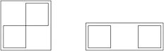
Figure 4.5: A simple greedy strategy can produce much dead space.

The second strategy is less greedy in that it computes a tiling for each level. We will describe it first in 2D [Leutenegger et al. 97]. Again, let B be the set of bounding volumes on the topmost level so far constructed, with B = n . The algorithm first computes the center c ⁱ for each b ⁱ ˆˆ B . Then it sorts B along the x -axis with respect to . Now, the set B is split into vertical slices (again with respect to ). Now, each slice is sorted according to and subsequently split into tiles, so that we end up with k tiles (see Figure 4.6). Finally, all nodes in a tile are combined under one common parent, its bounding volume is combined, and the process repeats with a new set B .

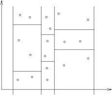
Figure 4.6: A less greedy strategy combines bounding volumes by computing a tiling.

In , it works quite similarly: we just split each slice repeatedly by along all coordinate axes.

Insertion. This construction scheme starts with an empty tree. Let B be the set of elementary bounding volumes. Algorithm 4.1 describes the general procedure.

Algorithm 4.1: Construction of BVHs by insertion.

 1:  while   B   >   do  2:          choose next  b     B  3:     := root 4:  while        leaf  do  5:                   choose child       ,                                  so that insertion of  b  into       causes minimal increase in the costs                             of the total tree 6:     :=       7:  end while  8:  end while

All insertion algorithms vary only Step 2 and/or 5. Step 2 is important because a bad choice in the beginning can probably never be made right afterwards. Step 5 depends on the type of query that is to be performed on the BVH. See the next section for a few criteria.

Usually, algorithms in this class have complexity O ( n log n ).

Top-down. This scheme is the most popular one. It seems to produce very good hierarchies while still being very efficient, and usually it can be implemented easily.

The general idea is to start with the complete set of elementary bounding volumes (which will become the leaves ), split that set into k parts, and create a BVH for each part recursively. The splitting should be guided by some heuristic or criterion that produces good hierarchies.

4.1.1. Construction Criteria

In the literature, there is a vast number of criteria for guiding the splitting, insertion, or merging during BVH construction. (Often, the authors endow the BVH thus constructed with a new name , even though the bounding volumes utilized are well known.) Obviously, the criterion depends on the application for which the BVH is to be used. In the following, we will present a few of these criteria.

For ray tracing, if we can estimate the probability that a ray will hit a child box when it has hit the parent box, we know how likely it is that we need to visit the child node when we have visited the parent node. Let us assume that all rays emanate from the same origin (see Figure 4.7). Then we can observe that the probability that a ray s hits a child box under the condition that it has hit the father box is

(4.1)

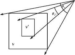
Figure 4.7: The probability of a ray hitting a child box can be estimated by the surface area.

where Area denotes the surface area of the BV, and denotes the solid angle subtended by the BV. This is because, for a convex object, the solid angle subtended by it, when seen from large distances, is approximately proportional to its surface area [Goldsmith and Salmon 87]. So, a simple strategy is to minimize the surface area of the bounding volumes of the children that are produced by a split. ^[1]

A more elaborate criterion tries to establish a cost function for a split and minimize that. For ray tracing, this cost function can be approximated by

(4.2)

where ₁ , ₂ are the children of . The optimal split B = B ₁ ˆ B ₂ minimizes this cost function:

where B ₁ ,B ₂ are the subsets of elementary bounding volumes (or objects) assigned to the children. Here, we have assumed a binary tree, but this can be extended to other arities analogously.

Of course, such a minimization is too expensive in practice, in particular, because of the recursive definition of the cost function. So,[Fussell and Subramanian 88, M