Chapter 4: Bounding Volume Hierarchies

Overview

In Chapter 3, we obtained a new data structure (BSPs) by starting from kd-trees and lifting one restriction, namely that splitting planes be always perpendicular to one of the coordinate axes. Starting again from kd-trees, we can regard them as a way to hierarchically group objects (points, polygons, etc.), rather than a way to partition space. In the simple kd-tree, all nodes on the same level partition space, and their extents are implicitly given by the path from the root. Since we now abandon this property, we can as well explicitly store the smallest bounding box enclosing all objects associated with a node, which is usually smaller than the extent of the kd-tree cell of that node. Thus, we have arrived at one particular type of bounding volume (BV) hierarchy.

Often times, bounding volume hierarchies (BVHs) are described as the opposite of spatial partitioning schemes, such as quadtrees or BSP trees: instead of partitioning space, the idea is to partition the set of objects recursively until some leaf criterion is met. However, we hope it has become clear by now that we regard BVHs as just one class of geometric data structures within the whole spectrum of hierarchical data structures.

Like the previous hierarchical data structures, BVHs are mostly used to prevent performing an operation exhaustively on all objects. Almost all queries that can be implemented with other space partitioning schemes can also be answered using BVHs. Examples of queries and operations are ray shooting, frustum culling, occlusion culling, point location, nearest neighbor, and collision detection (the latter will be discussed in more detail later in this chapter).

Definition 4.1. (BVH.)   Let O = { o ₁ , , o _n } be a set of elementary objects. A BVH for O , BVH( O ), is defined by

1. if O = e , then BVH( O ) := a leaf node that stores O and a bounding volume of O ;

2. if O > e , then BVH( O ) := a node with n ( ) children ₁ , , _n , where each child _i is a BVH, BVH( O _i ), over a subset O _i O , such that O _i = O . In addition, stores a BV of O .

The definition mentions two parameters. The threshold e is often set to 1, but depending on the application, the optimal e can be much larger. Just as in sorting, when the set of objects is small, it is often cheaper to perform the operation iteratively on all of them, because recursive algorithms always incur some overhead.

Another parameter in the definition is the arity. Mostly, BVHs are constructed as binary trees, but again, the optimum can be larger. And what is more, as the definition suggests, the out-degree of nodes in a BVH does not necessarily have to be constant, although this often simplifies implementations considerably.

Effectively, these two parameters, e and n ( ), control the balance between linear search/operation (which is exhaustive) and a maximally recursive algorithm.

There are more design choices possible according to the definition. For inner nodes, it requires only that O _i = O ; this means that the same object o ˆˆ O could be associated with several children. Depending on the application, the type of BVs, and the construction process, this may not always be avoidable. But if possible, you should split the set of objects into disjoint subsets .

Finally, there is at least one more design choice: the type of BV used at each node. This does not necessarily mean that each node uses the same type of BV. Figure 4.1 shows a number of the most commonly used BVs. The difference between OBBs [Arvo and Kirk 89] and AABBs is that OBBs can be orientedarbitrarily (hence oriented bounding boxes ). DOPs [Zachmann 98, Klosowski et al. 98, Kay and Kajiya 86] are a generalization of AABBs; basically, they are the intersection of k slabs. Prisms and cylinders have been proposed by [Barequet et al. 96] and [Weghorst et al. 84], but they seem to be too expensive computationally . A spherical shell is the intersection of a shell and a cone (the cones apex coincides with the spheres center), and a shell is the space between two concentric spheres. Finally, one can always take the intersection of two or more different types of BVs [Katayama and Satoh 97].

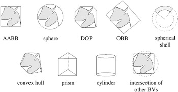
Figure 4.1: Some bounding volumes . (Courtesy of Blackwell Publishing.)

There are three characteristic properties of BVs: tightness, memory usage, and the number of operations needed to test the query object against a bounding volume.

Often, one must make a trade-off between these properties, because generally , the type of BV that offers better tightness also requires more operations per query and more memory.

Regarding the tightness, one can establish a theoretical advantage of OBBs. But first, we need to define tightness [Gottschalk et al. 96].

Definition 4.2. (Tightness by Hausdorff distance.)   Let B be a BV, and G be some geometry bounded by B , i.e., g B . Let

be the directed Hausdorff distance , i. e., the maximum distance of B to the nearest point in G . (Here, d is any metric, very often just the Euclidean distance.) Let

be the diameter of G .

Then we can define tightness as

See Figure 4.2 for an illustration.

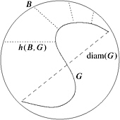
Figure 4.2: One way to define tightness is via the directed Hausdorff distance.

Since the Hausdorff distance is very sensitive to outliers, one could also think of other definitions such as the following one.

Definition 4.3. (Tightness by volume.)   Let C ( ) b the set of children of a node of the BVH. Let Vol( ) be the volume of the BV stored with .

Then we can define the tightness as

Alternatively, we can define it as

where L ( ) is the set of leaves beneath .

Getting back to the tightness definition based on the Hausdorff distance, we observe a fundamental difference between AABBs and OBBs [Gottschalk et al. 96] as follows .

• The tightness of AABBs depends on the orientation of the enclosed geometry. What is worse is that the tightness of the children of an AABB enclosing a surface of small curvature is almost the same as that of the parent.

  The worst case is depicted in Figure 4.3. The tightness of the parent is = h/d , while the tightness of a child is .

  
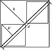
  Figure 4.3: The tightness of an AABB remains more or less constant xhroughout the levels of an AABB hierarchy for surfaces of small curvature.

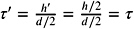
• The tightness of OBBs does not depend on the orientation of the enclosed geometry. Instead, it depends on its curvature, and it decreases approximately linearly with the depth in the hierarchy.

  Figure 4.4 depicts the situation for a sphere. The Hausdorff distance from an OBB to an enclosed spherical arc is h = r (1 ˆ cos ), while the diameter of the arc is d = 2 r sin . Thus, the tightness for an OBB bounding a spherical arc of degree is , which approaches 0 linearly as 0.

  
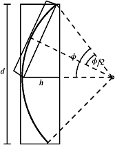
  Figure 4.4: The tightness of an OBB decreases for deeper levels in an OBB hierarchy for small curvature surfaces

This makes OBBs seem much more attractive than AABBs. The price of the much improved tightness is the higher computational effort needed for most queries per node when traversing an OBB tree with a query.