9.4 Advanced motion estimationcompensation

9.4 Advanced motion estimation/compensation

Motion estimation/compensation is probably the most evolutionary coding tool in the history of video coding. For every previous generation of video codecs, motion estimation has been considered as a means of improving coding efficiency. In the first video codec (H.120) under COST211, which was a DPCM-based codec, working on pixel-by-pixel, motion estimation for each pixel would have been costly and hence it was never used. Motion estimation was made optional for the H.261 block-based codec, on the grounds that the DCT of this codec is to decorrelate interframe pixels, and since motion compensation reduces this correlation, then nothing is left for DCT! Motion compensation in MPEG-1 was considered seriously, since for B-pictures, which refer to both past and future, the motion of objects even those hidden in the background can be compensated. It was so efficient that it was also recommended for P-pictures, and even with a half pixel precision. In MPEG-2, due to interlacing, a larger variety of motion estimation/compensation between fields and frames, or their combinations, was introduced. The improvement in coding efficiency was at the cost of additional overhead for delivering the motion vectors to the receiver. However, for MPEG-1 and 2, coding at a rate of 1–5 Mbit/s, this overhead is negligible, but the question is how this overhead can be justified for H.263 at a rate of 24 kbit/s or less? In fact, as we will see below, some extensions of H.263 recommend using smaller block sizes, which imply more motion vectors per picture and they even suggest motion estimation precision should be at a quarter or one eighth of a pixel. All these increase the motion vector overhead, which is very significant at a very low bit rate of 24 kbit/s.

The fact is that, if motion compensation is efficient, the motion compensated pictures may not need to be coded by the DCT. That is, these blocks are only represented by their motion vectors. In H.261 and MPEG1, we have seen a form of macroblock that was coded only by the motion vector, without coding the motion compensated error. However, if the expected video quality is low and the motion estimation is efficient, then we can see more of these macroblocks in a codec. This is in fact what is happening with motion compensation in H.263. In the following sections some improvements to motion estimation/compensation, in addition to those introduced for H.261, MPEG-1 and 2, will be discussed. At the end of this section a form of motion estimation that warps the picture for better compensation of complex motion will be introduced. Although this method is not a part of any form of H.263 nor is recommended for other video coding standards, there is no reason why we cannot have this form of motion estimation and compensation in the future video codecs.

9.4.1 Unrestricted motion vector

In the default prediction mode of H.263, motion vectors are restricted so that all pixels referenced by them are within the coded picture area. In the optional unrestricted motion vector mode this restriction is removed and therefore motion vectors are allowed to point outside the picture [25-D]. When a pixel referenced by a motion vector is outside of the coded picture area, an edge pixel is used instead. This edge pixel is found by limiting the motion vector to the last full pixel position inside the coded picture area. Limitation of the motion vector is performed on a pixel-by-pixel basis and separately for each component of the motion vector.

9.4.2 Advanced prediction

The optional advanced prediction mode of H.263 employs overlapped block matching motion compensation and may have four motion vectors per macroblock [25-F]. The use of this mode is indicated in the macroblock-type header. This mode is only used in combination with the unrestricted motion vector mode [25-D], described above.

9.4.2.1 Four motion vectors per macroblock

In H.263, one motion vector per macroblock is used except in the advanced prediction mode, where either one or four motion vectors per macroblock are employed. In this mode, the motion vectors are defined for each 8 × 8 pixel block. If only one motion vector for a certain macroblock is transmitted, this is represented as four vectors with the same value. When there are four motion vectors, the information for the first motion vector is transmitted as the codeword MVD (motion vector data), and the information for the three additional vectors in the macroblock is transmitted as the codeword MVD_2-4.

The vectors are obtained by adding predictors to the vector differences indicated by MVD and MVD_2-4, as was the case when only one motion vector per macroblock was present (see section 9.1.2). Again, the predictors are calculated separately for the horizontal and vertical components. However, the candidate predictors MV1, MV2 and MV3 are redefined as indicated in Figure 9.3.

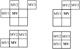
Figure 9.3: Redefinition of the candidate predictors MV1, MV2 and MV3 for each luminance block in a macroblock

As Figure 9.3 shows, the neighbouring 8 × 8 blocks that form the candidates for the prediction of the motion vector MV take different forms, depending on the position of the block in the macroblock. Note, if only one motion vector in the neighbouring macroblocks is used, then MV1, MV2 and MV3 are defined as 8 x 8 block motion vectors, which possess the same motion vector as the macroblock.

9.4.2.2 Overlapped motion compensation

Overlapped motion compensation is only used for 8 × 8 luminance blocks. Each pixel in an 8 × 8 luminance prediction block is the weighted sum of three prediction values, divided by eight (with rounding). To obtain the prediction values, three motion vectors are used. They are the motion vector of the current luminance block and two out of four remote vectors, as follows:

• the motion vector of the block at the left or right side of the current luminance block

• the motion vector of the block above or below the current luminance block.

The remote motion vectors from other groups of blocks (GOBs) are treated the same way as the remote motion vectors inside the GOB.

For each pixel, the remote motion vectors of the block at the two nearest block borders are used. This means that for the upper half of the block the motion vector corresponding to the block above the current block is used, and for the lower half of the block the motion vector corresponding to the block below the current block is used, as shown in Figure 9.4. In this Figure, the neighbouring pixels closer to the pixels in the current block take greater weights.

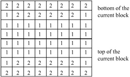
Figure 9.4: Weighting values for prediction with motion vectors of the luminance blocks on top or bottom of the current luminance block, H₁ (i, j)

Similarly, for the left half of the block, the motion vector corresponding to the block at the left side of the current block is used, and for the right half of the block the motion vector corresponding to the block at the right side of the current block is used, as shown in Figure 9.5.

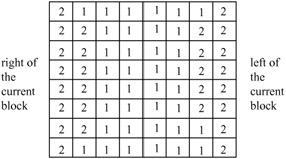
Figure 9.5: Weighting values for prediction with motion vectors of luminance blocks to the left or right of current luminance block, H₂(i, j)

The creation of each interpolated (overlapped) pixel, p(i, j), in an 8 × 8 reference luminance block is governed by:

(9.3)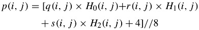 

where q(i, j), r(i, j) and s(i, j) are the motion compensated pixels from the reference picture with the three motion vectors defined by:

where denotes the motion vector for the current block, denotes the motion vector of the block either above or below and denotes the motion vector of the block either to the left or right of the current block. The matrices H₀(i, j), H₁(i, j) and H₂(i, j) are the current, top-bottom and left-right weighting matrices, respectively. Weighting matrices of H₁(i, j) and H₂(i, j) are shown in Figures 9.4 and 9.5, respectively, and the weighting matrix for prediction with the motion vector of the current block, H₀(i, j), is shown in Figure 9.6.

Figure 9.6: Weighting values for prediction with motion vector of current block, H₀(i, j)

If one of the surrounding blocks is not coded or is in intra mode, the corresponding remote motion vector is set to zero. However, in PB frames mode (see section 9.5), a candidate motion vector predictor is not set to zero if the corresponding macro block is intra mode.

If the current block is at the border of the picture and therefore a surrounding block is not present, the corresponding remote motion vector is replaced by the current motion vector. In addition, if the current block is at the bottom of the macroblock, the remote motion vector corresponding with an 8 × 8 luminance block in the macroblock below the current macroblock is replaced by the motion vector for the current block.

9.4.3 Importance of motion estimation

In order to demonstrate the importance of motion compensation and to some extent the compression superiority of H.263 over H.261 and MPEG-1, in an experiment the CIF test image sequence Claire was coded at 256 kbit/s (30 frames/s) with the following encoders:

• H.261

• MPEG-1, with a GOP length of 12 frames and two B-frames between the anchor pictures, i.e. N = 12 and M = 3 (MPEG-GOP)

• MPEG-1, with only P-pictures, i.e. N = ∞ and M = 1 (MPEG-IPPPP...)

• H.263 with advanced mode (H.263-ADV).

Figure 9.7 illustrates the peak-to-peak signal-to-noise ratio (PSNR) of the coded sequence. At this bit rate, the worst performance is that of MPEG-1, with a GOP structure of 12 frames per GOB, and two B-frames between the anchor pictures, (IBBPBBPBBPBBIBB...). The main reason for the poor performance of this codec at this bit rate is that I-pictures consume most of the bits and, compared with the other coding modes, relatively lower bits are assigned to the P and B-pictures.

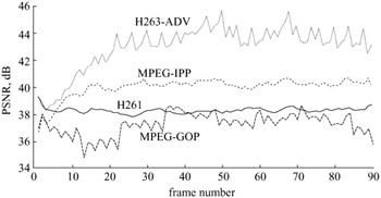
Figure 9.7: PSNR of Claire sequence coded at 256 kbit/s, with MPEG-1, H.261 and H.263

The second poorest is the H.261, where all the consecutive pictures are interframe coded with an integer pixel precision motion compensation. The second best performance is the MPEG-1 with only P-pictures. It is interesting to note that this mode is similar to H.261 (every frame is predictively coded), except that motion compensation is carried out with half pixel precision. Hence this mode shows the advantage of using half pixel precision motion estimation. The amount of improvement for the used sequence at 256 kbit/s is almost 2 dB.

Finally, the best performance comes from the advanced mode of H.263, which results in an almost 4 dB improvement over the best of MPEG-1 and 6 dB over H.261. The following are some of the factors that may have contributed to such a good performance:

• motion compensation on smaller block sizes of 8 x 8 pixels results in smaller error signals than for the macroblock compensation used in the other codecs

• overlapped motion compensation; by removing the blocking artefacts on the block boundaries, the prediction picture has a better quality, so reducing the error signal, and hence the number of significant DCT coefficients

• efficient coding of DCT coefficients through three-dimensional (last, run, level)

• efficient representation of the combined macroblock type and block patterns.

Note that, in this experiment, other options such as PB frames mode, arithmetic coding etc. were not used. Had the arithmetic coding been used, it is expected that the picture quality would be further improved by 1–2 dB. Experimental results have confirmed that arithmetic coding has approximately 5–10 per cent better compression efficiency over the Huffman [10].

9.4.4 Deblocking filter

At very low bit rates, the blocks of pixels are mainly made of low frequency DCT coefficients. In these areas, when there is a significant difference between the DC levels of the adjacent blocks, they appear as block borders. At the extreme case pictures break into blocks, and the blocking artefacts can be very annoying.

The overlapped block matching motion compensation to some extent reduces these blocking artefacts. For further reduction in the blockiness, the H.263 specification recommends deblocking of the picture through the block edge filter [25-J]. The filtering is performed on 8 × 8 block edges and assumes that 8 × 8 DCT is used and the motion vectors may have either 8 × 8 or 16 × 16 resolution. Filtering is equally applied to both luminance and chrominance data and no filtering is permitted on the frame and slice edges.

Consider four pixels A, B, C and D on a line (horizontal or vertical) of the reconstructed picture, where A and B belong to block 1 and C and D belong to a neighbouring, block 2, which is either to the right of or below block 1, as shown in Figure 9.8.

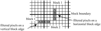
Figure 9.8: Filtering of pixels at the block boundaries

In order to turn the filter on for a particular edge, either block 1 or block 2 should be an intra or a coded macroblock with the code COD = 0. In this case B₁ and C₁ replace values of the boundary pixels B and C, respectively, where:

(9.4)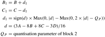 

The amount of alteration of pixels, ±d₁, is related to a function of pixel differences across the block boundary, d, and the quantiser parameter Q_P, as shown in eqn. 9.4. The sign of d₁ is the same as the sign of d.

Figure 9.9 shows how the value of d₁ changes with d and the quantiser parameter Q_P, to make sure that only block edges which may suffer from blocking artefacts are filtered, and not the natural edges. As a result of this modification, only those pixels on the edge are filtered so that their luminance changes are less than the quantisation parameter, Q_P.

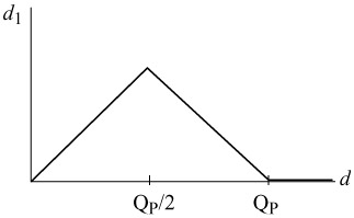
Figure 9.9: d₁ as a function of d

9.4.5 Motion estimation/compensation with spatial transforms

The motion estimation we have seen so far is based on matching a block of pixels in the current frame against a similar size block of pixels in the previous frame, the so-called block matching algorithm (BMA). It relies on the assumptions that the motion of objects is purely translational and the illumination is uniform, which of course are not realistic. In practice, motion has a complex nature that can be decomposed into translation, rotation, shear, expansion and other deformation components and the illumination changes are nonuniform. To compensate for these nonuniform changes between the frames a block of pixels in the current frame can be matched against a deformed block in the previous frame. The deformation should be such that all the components of the complex motion and illumination changes are included.

A practical method for deformation is to transform a square block of N × N pixels into a quadrilateral of irregular shape, as shown in Figure 9.10.

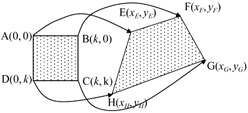
Figure 9.10: Mapping of a block to a quadrilateral

One of the methods for this purpose is the bilinear transform, defined as [11]:

(9.5) 

where a pixel at a spatial coordinate (u, v) is mapped onto a pixel at coordinate (x, y). To determine the eight unknown mapping parameters α₀-α₇, eight simultaneous equations relating the coordinates of vertices A, B, C and D into E, F, G and H of Figure 9.10 must be solved. To ease computational load, all the coordinates are offset to the position of coordinates at u = 0 and v = 0, as shown in the Figure. Referring to the Figure, the eight mapping parameters are derived as:

(9.6) 

where k = N - 1 and N is the block size, e.g. for N = 16, k = 15.

To use this kind of spatial transformation as a motion estimator, the four corners E, F, G and H in the previous frame are chosen among the pixels within a vertex search window. Using the offset coordinates of these pixels in eqn. 9.6, the motion parameters that transform all the pixels in the current square macroblock of ABCD into a quadrilateral are derived. The positions of E, F, G and H that result in the lowest difference between the pixels in the quadrilateral and the pixels in the transformed block of ABCD are regarded as the best match. Then α₀-α₇ of the best match is taken as the parameters of the transform that define the motion estimation by spatial transformation.

It is obvious that in general the number of pixels in the quadrilateral is not equal to the N² pixels in the square block. To match these two unequal size blocks, the corresponding pixel locations of the square block in the quadrilateral must be determined. Since these in general do not coincide with the pixel grid, their values should be interpolated from the intensity of their four surrounding neighbours, I₀, I₁, I₂ and I₃, as shown in Figure 9.11.

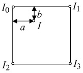
Figure 9.11: Intensity interpolation of a nongrid pixel

The interpolated intensity of the mapped pixels, I, from its four immediate neighbours, is inversely proportional to their distances and is given by:

(9.7) 

which is simplified to

I = (I₁ - I₀)a + (I₂ - I₀)b + (I₀ + I₃ - I₁ - I₂)ab + I₀

where a and b are the horizontal and vertical distances of the mapped pixel from the pixel with intensity I₀.

Note that this type of motion estimation/compensation is much more complex than the simple block matching. First, in block matching for a maximum motion speed of ω pixel/frame, there are (2ω + 1)² matching operations, but in the spatial transforms, since each vertex is free to move in any direction, the number of matching operations becomes (2ω + 1)⁸. Still each operation is more complex than BMA, since for each match the transformation parameters α₀-α₇ have to be calculated, and all the mapped pixels should be interpolated.

There are numerous methods of simplifying the operations [11]. For example, a fast matching algorithm, like the orthogonal search algorithm (OSA) introduced in section 3.3, can be used. Since for a motion speed of eight pixels/frame OSA needs only 13 operations, the total number of search operations becomes 13⁴ = 28 561, which is practical and is much less than using the brute force method of (2 × 8+1)⁸ = 7 × 10⁹, which is not practical! Also, the use of simplified interpolation reduces the interpolation complexity to some extent [12].

In order to appreciate the motion compensation capability of this method, a head-and-shoulders video sequence was recorded, at a speed of almost 12 frames per second, where the head moves from one side to another in three seconds. Assuming that the first frame is available at the decoder, the remaining 35 frames were reconstructed by the motion vectors only, and no motion compensated error was coded. Figure 9.12 shows frames 5, 15, 25 and 35 of the reconstructed pictures by the bilinear transform, called here block matching with spatial transform (BMST) and the conventional block matching algorithm (BMA). At frame 5, where the eye should be closed, the BMA cannot track it as this method only translates the initial eye position of frame one, where it was open, but BMST tracks it well. Also throughout the sequence, the BMST tracks all the eye's and head's movements (plus opening and closing the mouth) and produces almost good quality picture, but BMA produces a noisy image.

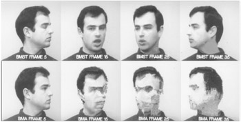
Figure 9.12: Reconstructed pictures with the BMST and BMA motion vectors operating individually

To explain why the BMST can produce such a remarkable performance, consider Figure 9.13, where the reconstructed pictures around frame 30, i.e. frames, 28–32, are shown. Looking at the back of the ear, we see that from frame to frame the hair grows, such that at frame 32 it looks quite natural. This is because if, for example, the quadrilateral is only made up of a single black dot, and it is then interpolated over the 16 × 16 pixels, to be matched to the current block of the same size in hair, then the current block can be made from a single pixel.

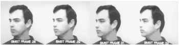
Figure 9.13: Frame by frame reconstruction of the pictures by BMST

Note that in BMST, each block requires eight transformation parameters equal to four motion displacements at the four vertices of the quadrilateral. Either the eight parameters α₀-α₇ or four displacement vectors at the four vertices of the quadrilateral as four motion vectors should be sent. The second method is preferred, since α₀-α₇ are in general noninteger values and need more bits than the four motion vectors. Hence, the motion vector overhead of this method is four times that of BMA for the same block size. However, if BMA of 8 × 8 pixels is used as in the advanced prediction mode [25-F], then we have the same overhead. Again this is irrespective of the block size, since BMA compensates for translational motion only, and cannot produce any better results than those above.

One way of reducing the motion vector overhead is to force the vertices of the four adjacent quadrilaterals to a common vertex. This generates a net-like structure or mesh, as shown in Figure 9.14a. As can be seen, the motion compensated picture (Figure 9.14b) is smooth and free from blocking artefacts.

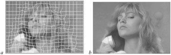
Figure 9.14: Mesh-based motion compensation (a mesh) (b motion compensated picture)

To generate such a mesh, the three vertices of a quadrilateral are fixed to their immediate neighbours and only one (bottom right vertex) is free to move. This constrains the efficiency of the motion estimation and for better performance motion estimation for the whole frame has to be iterated several times. Thus it is not expected to perform as well as the unconstrained movement of the vertices applied to Figure 9.12. Despite this, since mesh-based motion estimation creates a smooth boundary between the quadrilaterals, the motion compensated picture will be free from blockiness. Also, it needs only one motion vector per quadrilateral, similar to BMA. Thus this mesh-based motion estimation is expected to be better than the BMA with the same motion vector overhead, but of course with increased computational complexity. Figure 9.15 compares the motion compensation efficiency of the full search block matching algorithm (BM-FSA) with quadrilateral matching, using three-step search (QM-TSS) and the mesh-based iterative algorithm (MB-ITR). The motion compensation is applied between the incoming pictures, to eliminate accumulation of errors. Also, since QM requires four motion vectors per block, in order to reduce motion vector overhead, each macroblock is first tested with BMA, and if the MBA motion compensated error is larger than a given threshold, QM is used, otherwise BMA is used. Hence the MQ overhead is less than four times that of BMA. Our investigations show that for head-and-shoulders type pictures, about 20–30 per cent of the macroblocks need QM and the rest can be faithfully compensated by the BMA method. In this Figure, QM also used overlap motion compensation [13]. However, the mesh-based (MB) method, requires the same overhead as for BMA (slightly less, no need at the picture borders).

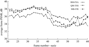
Figure 9.15: Performance of spatial transform motion compensation

As the Figure shows, mesh-based motion compensation is superior to the conventional block matching technique, with the same motion vector overhead. Considering the smooth motion compensated picture of the mesh-based method (Figure 9.14) and its superiority over block matching, it is a good candidate to be used in standard codecs.

More information on motion estimation with spatial transforms is given in [11,14,15]. In these papers some other spatial transforms such as Affine and Perspective are also tested. Methods for their use in a video codec to generate equal overhead to those used in H.263 are also explained.