Geometric Datatypes and gnuplotA Simple Example
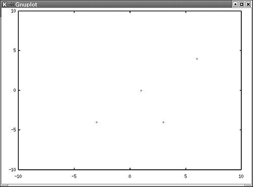
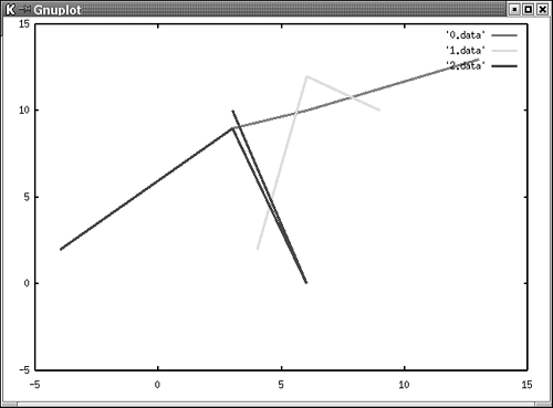
Geometric Datatypes and gnuplot ”A Simple ExamplePostgreSQL supports a powerful set of geometric datatypes. Displaying geometric data stored in a PostgreSQL database for many applications might be useful. Drawing database-driven images can be a difficult task, although there is a lot of Unix software available to do the job. Gimp, for instance, provides a powerful ASCII interface to generate and manipulate images from the command line (which is useful for Web applications). You also can use a scripting language in combination with gnuplot to do the job. This section shows you some basic ideas for visualizing geometric data stored in a PostgreSQL database. Let's start with a simple example. We have compiled a small table containing some points: mygnuplot=# SELECT * FROM mypoints; mypoints ---------- (1,0) (6,4) (-3,-4) (3,-4) (4 rows) With the help of a trivial shell script, we can generate a simple plot. Before we get to the gnuplot code, here is the shell script that we will use to transform the data to the desired format: #!/bin/sh psql -c 'SELECT * FROM mypoints' -t mygnuplot sed -e 's/,/ /gi' -e 's/)/ /gi' -e 's/(/ /gi' First we select the data from table gnuplot . -t makes sure that only the data is returned by the query. In the next step, we use sed (stream editor) to parse the data. We eliminate all brackets and commas so that gnuplot can easily read the input. Then we start gnuplot and use some simple commands: gnuplot> set nokey gnuplot> set xrange [-10 : 10] gnuplot> set yrange [-10 : 10] gnuplot> plot '< /home/hs/geo/plot.sh' The first three lines define some basic properties of the graph, such as the range of values displayed on the x-axis. The fourth line starts our shell script and sends the data to gnuplot. Figure 20.10 shows the display when you run gnuplot. Figure 20.10. Drawing points. The next example demonstrates how polygons can be plotted with the help of gnuplot. We have already dealt with polygons in Chapter 3, "An Introduction to SQL;" this time we generate a simple prototype of a script that prints all polygons stored in the table in a graph. We have compiled a small table containing three polygons: mygnuplot=# SELECT * FROM mypolygons; mypolygons ------------------------------- ((-4,2),(3,9),(6,10),(13,13)) ((4,2),(5,7),(6,12),(9,10)) ((-4,2),(3,9),(6,0),(3,10)) (3 rows) The following source code is a small script generating a config file for gnuplot: #!/usr/bin/perl use DBI; # connecting $connect="dbi:Pg:dbname=mygnuplot;port=5432"; $dbh=DBI->connect("$connect","hs") or die "cannot connect to the database\ n"; # getting lines $sql="SELECT * FROM mypolygons"; $sth=$dbh->prepare("$sql") or die "cannot prepare statement\ n"; $sth->execute() or die "cannot execute query\ n"; # open gnuplot config-file open(PLOT,"> config.plot") or die "cannot open config file for gnuplot\ n"; print PLOT "set xrange [-5 : 15]\ n"; print PLOT "set yrange [-5 : 15]\ n"; # setting variables and retrieving data $files=0; $plotstring="plot"; while (@row = $sth->fetchrow_array) { $line=$row[0]; $line=~s/\ ),\ (/\ n/gi; $line=~s/\ (\ )//gi; $line=~s/,/ /gi; # open file that contains data open(DATA,"> $files.data") or die "cannot open file $files.data\ n"; print DATA "$line\ n"; close(DATA); # generating plot command $plotstring.=" '$files.data' with lines linewidth 3,"; $files++; } $plotstring=~s/,$//gi; print PLOT "$plotstring\ n"; close(PLOT); # drawing data and cleanups system("gnuplot -background white -persist config.plot"); system("rm -f [0-9].data"); First we connect to the database and send a simple SQL query to the server that retrieves all records in table mypolygons . As you learned in Chapter 9, "Extended PostgreSQL ”Programming Interfaces," the SQL query has to be prepared and executed to receive the required result. Then we open the file, called config.plot , that we need to store the gnuplot code: $files=0; $plotstring="plot"; These two lines initialize two important variables. $files contains the number of polygons our graph will contain. $files is also used for generating the temporary file. $plotstring contains the plot command for our graph. Every polygon added to the scenery requires its own entry in the plot command. After initializing the variables, we start retrieving the data from the query that we have processed before. Every line returned will be transformed to the required format and stored in a temporary file. After that, the polygon is added to the scenery: We extract the line from the result of our query and perform some basic operation such as substituting ),( for a linefeed . This is necessary so that gnuplout can distinguish the various points of our polygon. We also eliminate all other brackets by using simple regular expressions. After adding all components to the graph, we substitute the comma at the end of $plotstring for nothing and write the string to the file. Our config file is now ready and we can execute gnuplot using the file. Before we have a look at the graph, we have included the file config.plot. You can see that the plot command consists of three components, each having its own datafile: set xrange [-5 : 15] set yrange [-5 : 15] plot '0.data' with lines linewidth 3, '1.data' with lines linewidth 3, '2.data' with lines linewidth 3 The most important component of our program is the converter that we use for reformatting the output of the database to a format that we can use for gnuplot. Recall that you do this with regular expressions. Lines such as the next one are converted to a file containing multiple lines: ((-4,2),(3,9),(6,10),(13,13)) Every node of the polygon is transformed to a separate line: -4 2 3 9 6 10 13 13 Keep in mind, that the columns of the file should be separated by a blank or a tab; if you use commas, gnuplot will not display the result correctly (if you don't define an input format). Figure 20.11 shows the graph. Figure 20.11. Drawing the polygons stored in the database. Three polygons are displayed, because three records have been retrieved from the database. As you can see, drawing database-driven geometric objects is an easy task with gnuplot. Of course it is not only possible to implement converters for points and geometric objects. Because gnuplot is flexible and powerful, it is possible to draw almost anything ”just try it. |
- ERP Systems Impact on Organizations
- Enterprise Application Integration: New Solutions for a Solved Problem or a Challenging Research Field?
- The Effects of an Enterprise Resource Planning System (ERP) Implementation on Job Characteristics – A Study using the Hackman and Oldham Job Characteristics Model
- Healthcare Information: From Administrative to Practice Databases
- A Hybrid Clustering Technique to Improve Patient Data Quality