4. Performance

4. Performance

In this section, we show simulations of the clustering algorithms for rate adaptive merging described earlier, and compare them with some heuristic algorithms that are described later in this section.

4.1 Objective

Some of the algorithms described in Section 2 are optimal in the static case (i.e., in the absence of user interactions). In addition, no optimal algorithms are known for the dynamic scenario in which users arrive into the VoD system, interact and depart. However, the behavior of such a system with the application of the aforementioned clustering and merging techniques can be studied by simulations. In these simulations, we investigate the gains offered by an ensemble of techniques under varying conditions. We attempt to answer the following questions:

• Which policy is best in the non-interactive scenario?

• Which policy is best under dynamic conditions in the long run?

• What is the effect of high arrival and interaction rates on these algorithms?

• What algorithm should be used when facing server overload?

4.2 The Simulation Setup

We treat the simulation as a discrete-time control problem. As outlined in Section 2, there are various ways in which we can control the system including: apply control with a fixed frequency, apply control with a fixed event frequency or adapt control frequency depending on the event frequency. The last technique is the hardest to implement. In this work, we have considered only the first method of periodic application of control.

The simulation set up consists of two logical modules: a discrete event simulation driver and a clustering unit. The simulation driver maintains the state of all streams and generates events for user arrivals, departures and VCR actions (fast-forward, rewind, pause and quit) with inter-event times obeying an exponential probability distribution. Here we have not considered a bursty model of interactions. A merging window (also called the re-computation period) is an interval of time within which a clustering algorithm attempts to release channels. Once every re-computation period, the simulation driver conveys the status of each stream to the clustering unit and then queries it after every simulation tick to obtain each stream's status according to the specified clustering algorithm. It then advances each stream accordingly. For instance, if the clustering unit reports the status of a particular stream to be accelerating at a given instant of time, the simulation driver advances that stream at a slightly faster rate of times that of a normal-speed stream.

The clustering unit obtains the status of all running streams from the simulation driver and computes and stores the complete merging tree for every cluster in its internal data structures until it is asked to recompute the clusters. On this basis, it supports querying on the status of any running non-interacting stream by the simulation driver after every simulation time unit.

4.3 Assumptions and Variables

The main parameters in our simulations are listed in Table 37.2. We simulated three types of interactions: fast forward, rewind and pause. λ_int is an individual parameter that denotes the rate of occurrence of each of the above interaction types (e.g., if λ_int= 0.02 sec^-1, it means a fast-forward or a rewind, etc. occurs in the system once every 50 seconds). For simplicity we maintain λ_int the same for each type of interaction.

Table 37.2: Simulation Parameters

Parameter	Meaning	Value
M	Number of movies [2]	100
L	Length of a movie	30 min
W	Re-computation window	10–1000 sec
λarr	Mean arrival rate [3]	0.1, 0.3, 0.7, 1.0 sec-1
λint	Mean interaction Rate[3], [4]	0, 0.01, 0.1 sec-1
λdur	Mean interaction time[3]	5 sec
[2]Movie popularities obey Zipf's law. [3]Exponential distribution assumed. [4]for each type of interaction.

λ_arr and λ_int determine the number of users in the system at any given time. The user pool is assumed to be large. Also, we do not consider the probability of blocking of a requesting user here as we assume that the capacity of the system is greater than the number of occupied channels.

The content progression rate of a normal speed stream is set at 30 fps and that of an accelerated stream is 32 fps. The accelerated rate can be achieved in practice by dropping a B picture from every MPEG group of pictures while maintaining a constant frame play-out rate. Fast-forward and fast-rewind are fixed at 5X normal speed. Finally, the simulation granularity is 1 sec and the simulation duration is 8,000 sec.

We investigated the channel and bandwidth reclamation rates for each clustering algorithm and compared the results (Section 4.5).

4.4 Clustering Algorithms and Heuristics

We simulated six different aggregation policies and compared them:

EMCL-RSMA Clusters are formed by the EMCL algorithm, and then merging is performed in each cluster by the RSMA-slide algorithm (Section 2).

EMCL-AFL Clusters are formed by the EMCL algorithm, and then merging is performed by forcing all trailers in a cluster to chase their cluster leader.

EMCL-RSMA-heuristic Clusters are formed by the EMCL algorithm, and then merging is performed by a RSMA-heuristic which is computationally less expensive than the RSMA-slide algorithm.

RSMA The RSMA-slide algorithm is periodically applied to the entire set of streams over the full length of the movie, but without performing EMCL for clustering.

RSMA-heuristic The RSMA-heuristic algorithm is periodically applied to the entire set of streams over the full length of the movie, but without performing EMCL for clustering.

Greedy-Merge-heuristic Merging is done in pairs starting from the top (leading stream) in the sorted list. If a trailer cannot catch up to its immediate leader within the specified window, the next stream is considered. At every merge, interaction, or arrival event, a check is performed to determine if the immediate leader is a normal speed stream. If so, and merging is possible within a specified window, the trailing stream is accelerated towards the immediate leader. This process is continued throughout the window. GM is similar to Golubchik's heuristic [11] apart from the fact that it re-evaluates the situation at every interaction event as well.

The first three policies release the same number of channels at the end of an interval because they use the EMCL algorithm for creating mergeable clusters. But, the amount of bandwidth saved in the merging process is different in each case. EMCL-RSMA proves to be optimal over a given merging window, so it conserves the maximum bandwidth. EMCL-AFL is a heuristic and can perform poorly in many situations. EMCL-RSMA-heuristic, in contrast, uses an approximation algorithm for the RSMA-slide that guarantees a solution within twice the optimal [19]. Although our problem falls within the slide category and has an O(n³) exact solution, we experiment with the approximation algorithm that runs in O(n log n) time.

4.5 Results and Analysis

Here we discuss clustering gains (channel reclamation) and merging gains (bandwidth reclamation) due to the aforementioned algorithms. We classify the simulations into two categories:

4.5.1 Static Snapshot Case

The static snapshot case is applicable in overload situations. That is, when the server detects an overload, it wants to release as many channels as possible in a static merging window (one in which there are no user interactions). We vary the window size for a fixed number of users. Figure 37.7(a) shows that the clustering gain increases as W increases. Also visible is that EMCL outperforms GreedyMerge over any static window of size W. Figure 37.7(b) compares the bandwidth gains due to the three merging algorithms. The merging gain increases with increase in W. Also, over any static window in the graph, the gains due to EMCL-RSMA and EMCL-RSMA-heur are almost identical! Although EMCL-RSMA is provably optimal over a static window, the RSMA heuristic does as well in most cases (the reason for this may be attributed to the parameters of the particular inter-arrival distribution). Although cases can be constructed in which the heuristic produces a result that is twice the optimal value, in most practical situations it performs as well as the exact algorithm at a lower computational cost.

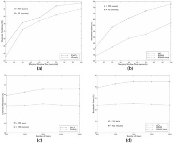
Figure 37.7: Static snapshot case.

Figure 37.7(c) shows the number of users varied for a fixed window size of 100 s comparing GM and EMCL. Clearly, EMCL performs better than GM and their clustering gains remain almost constant throughout the curves although the gap between the two appears to increase as U increases. Figure 37.7(d) shows that EMCL-RSMA and its heuristic version perform equally well and clearly reclaim more bandwidth than EMCL-AFL. Even in this case, the percentage gains appear to remain constant as U increases.

4.5.2 Dynamic Case

The dynamic case is the general scenario in which users come into the system, interact and then leave. Here, we simulate over a time equivalent of approximately 4 1/2 lengths of the movies.

We study the behavior of cumulative channel reclamation gains due to the above algorithms as a function of time for cases with varying rates of user arrival and interactions. We considered 12 different arrival-interaction patterns as shown in Table 37.3.

Table 37.3: Arrival and Interaction Patterns

Arrivals/ Interactions	NO	LOW	HIGH
LOW	λarr =0.1, λint=0	λarr =0.1, λint =0.01	λarr =0.1, λint =0.1
LOW-MEDIUM	λarr =0.3, λint=0	λarr =0.3, λint =0.01	λarr =0.3, λint =0.1
HIGH-MEDIUM	λarr =0.7, λint =0	λarr =0.7, λint =0.01	λarr =0.7, λint =0.1
HIGH	λarr =1.0, λint =0	λarr =1.0, λint =0.01	λarr =1.0, λint =0.1

For each of the above cases and for each of the six different aggregation policies, we ran the simulations for eight different re-computation window sizes(W): 10, 25, 50, 100, 200, 500, 750 and 1,000 seconds. Figure 37.8 shows the steady-state behavior of the system for λ_arr = 0.7 and λ_int = 0.1. We can clearly see that RSMA outperforms all other policies by a large margin for small and medium values of W. For W = 100 sec, RSMA reclaims about 400 channels from 1,250 channels after the steady state is reached thus yielding gains of about 33%. This essentially means that for the particular type of traffic (λ_arr = 0.7 and λ_int = 0.1), we do not need more than 850 channels to serve 1,250 streams.

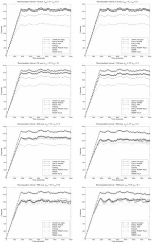
Figure 37.8: Dynamic clustering in steady state.

For smaller W, other policies provide diminished channel gains. But as the re-computation interval is increased, RSMA begins to suffer and EMCL based policies and GM begins to perform well. This is because RSMA takes a snapshot of the whole system at the beginning of a recomputation interval and advances streams according to the RSMA tree computed from that snapshot. In the situation in which the user arrival rate is moderately high and the interaction rate is high as well, for high values of W, many streams come in and interact between two consecutive snapshots and thus the gains due to RSMA drop. In contrast, GM tries to re-evaluate the situation at every arrival and interaction event, so it performs very well.

Our speculation and conclusion is that different policies will perform at their best for different values of W and, indeed, we found this to be true. Figure 37.9 shows how the channel gains vary with the value of the recomputation window. For consistency, we consider the case with λ_arr = 0.7 and λ_int = 0.1. The graphs for the other cases are similar in shape and have not been shown due to space limitations. In the steady state, the system has 1,250 users on average. For small values of W (≤ 500 sec.), EMCL-based schemes and GM do not perform well, whereas, RSMA and RSMA-heur perform well. However, for larger values of W (> 500 sec.), EMCL-based schemes and GM perform well and RSMA-heur is highly sub-optimal. Although RSMA shows reduced gains for higher values of W, it is still superior to EMCL-based algorithms. GM outperforms all algorithms, including RSMA for W ≥ 750 due to the reason mentioned in the previous paragraph. But GM is more CPU intensive as it reacts to every arrival, interaction, and merge event. In that sense, it is not a true snapshot algorithm like the others, and is not a scalable solution under heavy rates of arrival and interaction although it may perform better than the other algorithms in such situations.

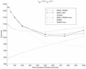
Figure 37.9: Dependence of channel gains on W.

Each policy attains its best results for different values of W. RSMA performs best for W = 10 sec; GM performs best for W = 1,000 sec. and the EMCL based algorithms perform best for 500 ≤ W ≤ 750. Figure 37.10 plots the best channel gain achieved by a policy for every class of traffic (see Table 37.3). In the figure, there are four sets of curves with three curves each. Each set corresponds to an arrival rate because λ_arr is the most dominant factor affecting the number of users in the system. The mean numbers of users in the system for λ_arr = 0.1, 0.3, 0.7 and 1.0 are 180, 540, 1,250 and 1,800, respectively. The mean clustering gains increase significantly with increase in the arrival rate.

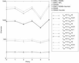
Figure 37.10: Comparison— With best W for each policy.

For each of the four sets, the channel gains are almost identical for λ_int = 0 and λ_int = 0.01 but are less for λ_int = 0.1. That is not far from expectations as a high degree of interaction causes each algorithm to perform worse. More importantly, the RSMA algorithm emerges as the best overall policy. As λ_arr increases, the gap between RSMA and the other algorithms widens.

Also, there is little difference in the gains due to EMCL-RSMA and its heuristic counterpart, although there is a vast difference between the gains due to RSMA and those due to the RSMA heuristic. This is because EMCL breaks a set of streams into smaller groups and the EMCL-RSMA heuristic performs almost identically well as EMCL-RSMA for smaller groups. But, in case of RSMA, the number of streams is large (EMCL has not been applied to the stream cluster), so the sub-optimality of the heuristic appears. Note that the RSMA-slide algorithm of complexity O(n³) is affordable in practical situations because it is invoked only once in every recomputation period. As a reference point, the running time of the algorithm on an Intel Pentium Pro 200 MHz PC running the Linux operating system is well below the time required to play out a video frame; therefore no frame jitter is expected on modern playback hardware.

From the above simulations, we conclude the following:

• EMCL-RSMA is the optimal policy in the static snapshot case as it reclaims the maximum number of channels with minimum bandwidth usage during merging. Thus it is the ideal policy for handling server overloads.

• In a VoD system showing 100 movies, for dynamic scenarios with moderate rates of arrival and interaction, periodically invoking RSMA with low re-computation periods yields the best results.

• In realistic VoD settings, the arrival rate plays a greater role than the interaction rate (except for interactive game settings where aggregation is not a feasible idea). High arrival rates result in more streams in the system thus creating better scope for aggregation.

• Higher degrees of interaction result in lesser clustering gains for every algorithm.

• With increasing rates of arrival, RSMA's edge over other algorithms increases.

• The EMCL-RSMA heuristic performs almost as well as EMCL-RSMA although the RSMA-heuristic performs very badly as compared to RSMA.

4.6 Comparisons between RSMA Variants

Here we compare the performance of the various forms of the RSMA-slide algorithm, namely, periodic snapshot RSMA (Slide), event-triggered RSMA (Section 2.6), stochastic RSMA (Section 3) and predictive RSMA (Section 2.6). We consider a single movie of length L = 2 hours.

First, we evaluate the performance of Slide in the "arrival-only" situation because it lends itself to easy comparison with the analytical framework described in Section 2.7. The behavior of the channel gains is depicted in Figure 37.11 (a) as a function of the recomputation interval R. The simulation results show that as R is increased, the channel gain degrades as a linear function of R. The analytically estimated channel gains as described in Section 2.7 are plotted on the same graph. From the graph we see that the analytical estimation comes reasonably close to the simulation results. Although the analytical technique underestimates the simulation results by approximately 10 streams, the slopes of the two curves are almost the same. The slope is very close to the analytical estimate of 1/2λ_a (Equation 37.11). The underestimation can be attributed primarily to the assumption that the recomputation results in formation of natural clusters, and the streams in two different clusters do not merge. This assumption may not be valid due to a possible effect of streams in one recomputation interval on those in the next or previous one.

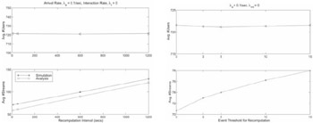
Figure 37.11: Two variants of RSMA.

Next, we consider the threshold based, event-triggered RSMA, in which recomputation is not done periodically but only when the number of events exceeds a threshold. Figure 37.11(b) shows the variation of the gains with the increase in the event count threshold. The case in which the threshold is 0 corresponds to the pure event-triggered RSMA where recomputation happens at the occurrence of each event. As expected, the gains decrease as the threshold is increased.

In summary, Table 37.4 shows the number of users and streams for each variant of RSMA in steady state. The Slide refers to the RSMA-slide with R = 10 sec. The rationale for using this value is that the arrival rate considered is 0.1 sec, and hence on average there will be an arrival every 10 seconds. By "perfect prediction," we intend the following: to evaluate whether gains are achieved with this technique that warrant obtaining the difficult prediction of future events. Note that the RSMA can be computed optimally under perfect prediction if the events comprise arrivals only, as shown in Section 2.4. When the actual stream arrives later, it just follows the path computed by the predictive RSMA algorithm. Stochastic RSMA reacts to every arrival event and the RSMA tree is determined using the technique described in Section 3. The event-triggered RSMA algorithm corresponds to the case in which the event count threshold is 0.

Table 37.4: Comparison between Variants of RSMA (λ_arr = 0.1, λ_int = 0, λ_q = 0)

RSMA Variant	Avg. #Users	Avg. #Streams	Avg. #Users per Stream
RSMA Slide (R = 10 sec)	722	71	10.17
Event Triggered RSMA	722	71	10.17
Predictive RSMA	721	71	10.15
Stochastic RSMA	732	137	5.34
GreedyMerge	720	373	1.93

We see from Table 37.4 that with the exception of the stochastic RSMA, the other variants perform almost identically under the current set of conditions. Because the merging algorithm alters the effective service time of a user by manipulation of the content progression rates, it affects the number of users in the system directly. The random number generator in the simulator produced user arrivals with mean λ_efrective = 0.1033/sec , which is slightly higher than the intended mean of λ_arr = 0.1/sec . Hence the average number of users in steady state in a non-aggregated system should be λ_effective L = 0.1033 7200 = 744, but due to aggregation, the effective service time for many streams is reduced when they progress in an accelerated fashion; hence the number of users in the system is reduced. Stochastic RSMA performs worse than the other RSMA variants because only the short-term cost is considered in the formulation. For comparison, we show the gains due to the deterministic "greedy" algorithm. It performs much worse than its stochastic greedy counterpart (i.e., stochastic RSMA) as well as the other RSMA variants.

Among all RSMA variants, the Slide is the simplest to implement and is computationally less expensive than its event-triggered counterpart because it does not react to every event. Predictive RSMA, in contrast, does not provide additional gains even with perfect prediction; hence the computational overhead involved in prediction is not justified. We conclude that the Slide algorithm yields the best results with the least computational overhead than its variants.

Figure 37.12 shows the effect of varying degrees of interactivity on the RSMA slide algorithm as a function of R in steady state. We considered three different values of interaction rates: 0, 0.01 and 0.02 per second for each type of interaction, respectively. The quit rate is held at a low constant value (0.001 per second) in order to prevent the number of users in the system from substantially varying. The linearity dependence on R is lost as the interaction rate increases - for λ_int = 0 , the curve is practically linear, whereas for λ_int = 0.02, the curve is not linear. This can be attributed to random interactions such as fast-forward and rewind result in greater fluctuations in stream positions at snapshots, thus making the merging trees of adjacent snapshots less correlated. Non-linearity arises in all three curves for lower values of R because there is no natural clustering due to taking snapshots with low R, and hence the streams in adjacent temporal clusters can merge later. Our analytical estimation framework does not take such behavior into account. As R increases, the gap between the interactive case and the non-interactive case widens significantly. This phenomenon is not unexpected as a larger R means more interaction events in that interval, which in turn translates to the increase in the loss of gains that were achieved due to merging. Hence, as observed before, high degrees of interactivity can be handled by recomputing the RSMA frequently.

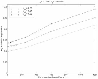
Figure 37.12: Effect of varying degrees of interactivity.

Table 37.5 shows the performance comparison of the different RSMA variants in the dynamic, interactive cases. In comparison with Table 37.4, the average number of users per stream is lower due to user interactions. The aggregate event rate is λ_arr + λ_int + λ_q = 0.161, and hence the mean inter-event time is 1/0.161 ≈ 6sec. Hence we use R = 6 in the RSMA-slide algorithm. The event-triggered RSMA performs slightly better than its slide counterpart, but not by a substantial margin. Expectedly, RSMA-slide with a slightly higher R (16 sec) yields slightly worse results than RSMA-slide with R = 6. However, Stochastic RSMA performs much worse as compared to the other variants because it does not take the long-term cost into account. The event triggered version of RSMA starts performing better than the periodic version as interactivity increases, but it has higher computational overhead. Therefore, a system designer should evaluate the system parameters and evaluate the trade-offs between the desired level of performance and computational overhead, and choose a clustering algorithm accordingly.

Table 37.5: Comparison between Variants of RSMA (λ_arr =0.1, λ_int = 0.01, λ_q = 0.001)

RSMA Variant	Avg. #Users per Stream
RSMA Slide (R = 6 sec)	8.33
RSMA Slide (R = 16 sec)	8.23
Event Triggered RSMA	8.62
Stochastic RSMA	4.23