Size the Kanban

Overview

In Chapter 3 you gathered data on your process in preparation for this point. In this chapter we will use the data from Chapter 3 to "size the kanban." Or, in layman's terms, you will determine how many containers of each product you will require to effectively operate the kanban (and keep your customer supplied). Figure 4-1 expands the model started in Figure 3-1 by adding this step.

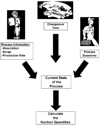
Figure 4-1: Calculating the Kanban Quantities .

Once you start kanban scheduling, these quantities become the maximum amount of inventory held. Therefore, when all these containers are full, then you stop production. This rule is one of the major tenets of kanban scheduling ”you only produce when you have signals.

These quantities become the scheduling signals. To set up these signals, we will determine the emergency level (or red level), the schedule signal (or yellow level), and the normal level (or green level). In Chapter 5 you will develop a kanban design, which uses these signals to control the production schedule.

In this chapter we propose two methods for sizing internal kanbans. The first method calculates the container quantities based on the data collected in Chapter 3. This method allows you to optimize and potentially reduce the quantities based on the characteristics of your process.

The second method uses your existing production schedule and makes the current production quantities the kanban quantities. This method allows for quicker implementation and less math, but does not offer the potential for reducing inventory levels.

We will discuss the benefits of each approach as we proceed through the chapter. However, our experience tells us that the first approach is better since it calculates the quantities based on the processes' capability. This method also typically leads to reduced inventory. We focus mainly on the calculation method, but also provide the information necessary to perform the second method. We will let you decide on which method to use for calculating your kanban quantities.

This chapter also addresses supplier kanbans. The primary issues with these kanbans will be safety stock and establishing the lead time for replenishment. As part of this activity we discuss kanbans with vendors who have already developed this type of scheduling system as well as kanbans with vendors who have no such experience. During the discussions about supplier kanbans, we show you a methodology for selecting the vendor parts that should be placed under kanban scheduling and how to address variability in order quantity. Additionally, Appendix H contains a case study that is based on a kanban in use at a plant with 3,000 different finished-goods part numbers , with batches as small as fifty units.

All of these initial kanban quantities should be based on your current condition instead of how you want the future to look. By using current data, you can start the kanban now, rather than waiting for your downtime, your scrap level, or your changeover times to be reduced.

Further, by using current data you reduce the risk of failure. Essentially when you size the kanban with wishful or projected future data, you open yourself up to raw material stock outs or production stoppages. Just like the case of overcompensating with buffers, sizing the kanban with future data creates an unreal production condition. Managers who make this mistake often wonder why every product is in the red level all the time.

Don't make the same mistake. Size the kanban with the current data, then set continuous improvement goals that will reduce the kanban quantities. Chapter 9 specifically addresses the various ways to reduce the kanban quantities. Best of all, these recommendations will be compatible with other Lean, or continuous improvement, activities you may already have underway.

Determining the Replenishment Cycle

In Chapter 3, we determined the scheduling interval and required production parts for the production process. We will refer to this cycle as the replenishment interval . It is the smallest batch size that your process can run and still keep the customer supplied. This interval essentially tells how long it takes to produce your adjusted production requirements. The replenishment interval is a function of the time available after considering your process parameter:

• Production rate
• Changeover times
• Downtime (both planned and unplanned )

The replenishment cycle will ultimately be determined by the time left over for changeovers after subtracting required production run time from available production time. Therefore, the length of this cycle will be a function of how long it takes to "bank" enough changeover time to make all the necessary changeovers.

These production requirements also need to account for your scrap. When the required parts include the scrap, then the term becomes your "adjusted requirements." These factors determine how many days, weeks, or months of inventory you keep on hand to supply the customer(s).

If this sounds confusing, then maybe some mathematical formulas will help. We'll start with calculating the adjusted production requirements. Adjusted production requirements are the quantity of a part that you must produce to cover the order quantity plus the system scrap. Mathematically, the equation for adjusted production requirements is shown in Figure 4-2.

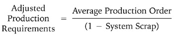
Figure 4-2: Equation for Adjusted Production Requirements Using the System Scrap.

For those production processes that must also account for downstream scrap (such as for in-house customers), then this equation changes to the equation in Figure 4-3.

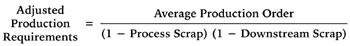
Figure 4-3: Equation for Adjusted Production Requirements When Scrap is Tracked as Process Scrap and Downstream Scrap.

You will need to make this calculation for each item produced by the process. By summing the adjusted production requirement for each part you will determine the total production quantity.

Note that you may not need to make the adjusted production requirements calculation if your normally scheduled quantity accounts for scrap in your production process and downstream. In fact, if this is the case, then taking the production quantities and adjusting for scrap with the equations in Figures 4-2 or 4-3 will only incorrectly increase the amount you need to produce ”i.e., by creating overproduction.

Once you know how much you have to produce, then you must determine how long it will take and how much time you have to produce it (each day, week, or month). The answers to these two questions will allow you to determine the time available for changeovers.

To determine how long it takes to produce the adjusted production requirements, you need to determine the time required for production of each part. To determine the time required for production, multiply the adjusted production requirements by the cycle time per part and sum for all the parts produced by the process. Mathematically, the equation for available time is shown in Figure 4-4.

Figure 4-4: Equation for Production Time.

Now calculate the available production time to determine how much time you have available each day to produce parts. While this may seem ridiculous since you have twenty-four hours in a day, available time refers to the time left after considering breaks, lunches, end of shift cleanup, shift starter meetings, equipment warm-up, breakdowns, kaizen activities, safety activities, PM downtime, etc. It is the time left over to produce parts. Mathematically, the equation for available time is shown in Figure 4-5.

Figure 4-5: Equation for Available Time.

Typically, most production processes have from 410 to 430 minutes of available time per shift. Once calculated, available time usually becomes a production standard.

If you operate a continuous process, then the equation for available time simply considers planned downtime for preventative maintenance/cleaning activities and breakdowns. Mathematically, the equation changes to the equation shown in Figure 4-6.

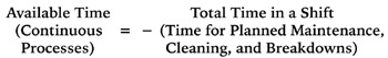
Figure 4-6: Equation for Available Time in a Continuous Process.

One source of confusion when calculating available time is how to allocate the time for events that do not occur every shift, such as safety meetings, kaizen activities, or preventative maintenance. To allocate time in the daily standard, simply determine the total time taken up by these events during a week or a month and divide by the shifts in a week or a month respectively. Once you have this number, simply subtract it from the total shift time. For example, if you allocate one hour per month for a safety meeting, one hour per week for kaizen and information meetings, and two hours per month for preventive maintenance (PM), total productive maintenance (TPM), and 5s cleaning, then the shift allocations would be calculated as shown in Figure 4-7.

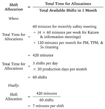
Figure 4-7: Allocating Improvement and Meeting Time for Available Time Calculations.

The final result of all this calculating will be the total time available for production requirements and changeovers. To determine the total time available for changeovers, subtract the time required for production from the total available. The mathematical equation is shown in Figure 4-8. The example in Figures 4-9 and 4-10 should clarify these calculations.

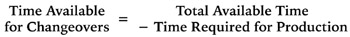
Figure 4-8: Equation for Time Available for Changeovers.

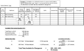
Figure 4-9: Calculating the Time Available for Changeovers for the Two-Part Number Example in Chapter 3.

Figure 4-10: Calculating the Time Available for Changeovers for the Ten-Part Number Example in Chapter 3.

Finally, you calculate the replenishment interval by determining the total time required for changeovers and dividing this number by the time available for changeovers. Mathematically, the equation is shown in Figure 4-11.

Figure 4-11: Equation for Replenishment Interval.

Taking our Figures 4-9 and 4-10 examples further, you can calculate the replenishment intervals for both production processes. Figures 4-12 and 4-13 show these calculations.

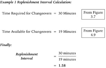
Figure 4-12: Calculation of Replenishment Interval for the Two-Part Number Example.

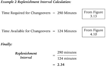
Figure 4-13: Calculation of Replenishment Interval for the Ten-Part Number Example.

Once you have the replenishment interval and lead times established, you multiply these numbers by the adjusted production interval requirements to determine the maximum number of parts in the kanban.

To determine the number of containers in the kanban, just divide the maximum kanban quantities by each part's container capacity. The container capacity will become the smallest unit of each part that you will produce. The total number of the containers then becomes the basis for determining the scheduling level and danger level.

Essentially, you will not receive a scheduling signal until the customer uses the replenishment interval quantity. (This quantity becomes the "green" level.) You then produce parts until you reach the part's maximum quantity. These assumptions should be tailored by the size of the kanban and specifics of your process. However, the fundamental rules of kanbans must be followed:

• Nothing is produced without a scheduling signal
• Production stops when no more signals exist

Implications of Scrap, Unplanned Downtime, and Changeover Times on Replenishment Intervals

If you remember, we started out this chapter by saying:

• Size your kanbans based on the current state of your production process.

This advice was based on our desire to help you avoid the agony of undersizing your kanban quantities , which can:

1. Cause you to continually operate at danger (or red) levels
2. Ultimately lead to your pronouncement of kanban as worthless and a waste of time

After seeing the calculation method, hopefully you see how scrap, unplanned downtime, and changeover times will drive the interval up or down. To illustrate this point, we varied scrap, downtime, and changeover time for the Figure 4-10 (or ten-part number) example. The graphs in Figures 4-14 to 4-17 show how the replenishment interval varies with the scrap, downtime, and changeover time changes.

Note that Figure 4-17 shows the benefits of an aggressive continuous improvement program that drives all of these values down. Because of the impact of these improvements, we have dedicated Chapter 9 to discussing improvements.

Calculating the Buffer

The last step in the process of sizing the kanban is to calculate your buffers. The buffers will provide you with the necessary lead time to produce the replenishment interval part quantities without stocking out your process or customer. The buffers also provide the necessary time required for process activities to occur. Buffer items that should be considered include:

• Customer delivery requirements (and your promised service)
• Internal lead times
• Supplier lead times
• Comfort level

Buffers should be considered in terms of how much inventory is needed to prevent the item from impacting the customer deliveries. The secret is to hold enough inventory to protect the customer without holding too much inventory.

Customer Delivery Requirements (and Your Promised Service)

The starting point for determining the buffer is the customer delivery requirements. Keeping the customer supplied should be the overriding driver in setting up the buffers. Therefore, the buffer must support the promised customer deliveries. So, when sizing the buffers for finished goods kanbans, make sure that you can deliver on the customer requirements (or your promises) in order to maintain customer satisfaction.

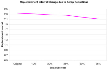
Figure 4-14: Impact of Scrap on Replenishment Intervals.

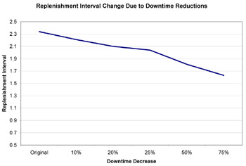
Figure 4-15: Impact of Scrap Unplanned Downtime on Replenishment Intervals.

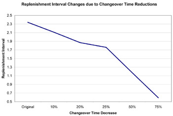
Figure 4-16: Impact of Changeover Times on Replenishment Intervals.

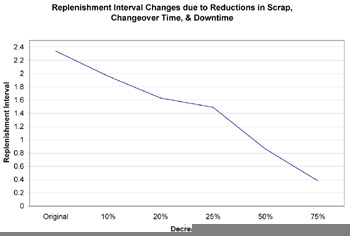
Figure 4-17: Impact of All Three Factors on Replenishment Intervals.

You can be aggressive with the internal and supplier buffers if you maintain a finished goods inventory buffer. The finished goods inventory can serve as the buffer for stock out of internal parts and supplier raw materials.

Internal Lead Times

Internal lead times refer to the process times to replenish parts. It also includes process constraints, such as chemical reaction times, cure or drying times, or inspections., Look at the process and size the buffer realistically to allow time for these activities to occur. Also, look at the lead times of your internal suppliers and factor in their lead times to resupply your process.

Supplier Lead Times

When looking at the lead times from the supplier, consider their production timeline as well as transportation time. Also, look at the supplier's reliability, quality, and delivery record when establishing their lead times. Don't pressure your suppliers into accepting unrealistic lead times. Don't put your production process in jeopardy (and ultimately customer service) by forcing fairytale commitments. To create a win-win environment, tell your supplier the target goals and let them accept the lead times.

When considering product transportation, also look at the transportation cost. You need to trade off the cost of holding inventory versus having more frequent deliveries. This analysis needs to consider the impact of partial shipments on your transportation budget and the space requirements to hold the larger quantity of material. (We will discuss options for minimizing freight costs due to partial shipments in Chapter 9.)

Comfort Level

Finally, determine your own desired inventory comfort level. Essentially, how much inventory do you need to sleep soundly at night? Here is where you need to be very careful that you don't let your desire for comfort make you into an inventory glutton.

When determining your inventory comfort level, use the previously collected data to challenge your beliefs about the necessary buffers. Is there fat in the process that causes you to overcompensate? What about any "hidden factory inventory" ”such as multiple containers of material being staged at a downstream operation while still maintaining a control point?

Once again, look at how large of buffer the current operation uses. If you're not carrying extra material now, then why will you need it in kanban scheduling? The buffer requirements will be an excellent discussion topic for the team.

Determining the Final Buffer Size

When you have addressed these items, determine a final number for your buffer. Realistically look at the various items and determine if the events will occur in series or randomly to determine the final number. Essentially, will the buffers be additive or will one quantity be sufficient.

Calculating the Number of Kanban Containers

When you have determined how much buffer you require, then you are ready to calculate the final kanban container quantities . To calculate the number of containers, add together the buffer quantity and the replenishment interval, then multiply this number by the adjusted production quantity, and finally divide by the container capacity. Figure 4-18 shows the mathematical equation.

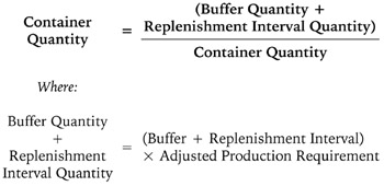
Figure 4-18: Equation for Calculating the Container Quantity.

To determine all the container quantities, repeat this calculation for each of the production part numbers produced by the process. Figures 4-19 and 4-20 show buffer assumptions and the container calculations for the examples in Figures 4-9 and 4-10.

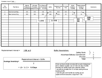
Figure 4-19: Container Calculations for the Example in Figure 4-9.

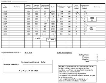
Figure 4-20: Container Calculations for the Example in Figure 4-10.

Perform a Reality Check

When your calculations are complete, the hard part is done. You now need to look at the results of these calculations and assess their reality. At this point don't let funky numbers stop the process. If you get results that look strange , then step back and look at the assumptions. Follow the steps outlined below to drive out the culprit.

When you look at the final calculations, ask yourself these questions:

• Do the calculated quantities look like my current process?
• Does the inventory remain the same or decrease?

If you answer No to one of these questions, then you need to review your data to determine how you arrived at these numbers. Conversely, if you answer Yes, then you should also check your data to determine whether the new quantities look is unrealistically low.

Some of the common pitfalls with initial calculations include:

• Container sizes force added inventory
• Incorrect production data ”production requirements, scrap, downtime, and changeovers
• Incorrect buffer assumptions
• Incorrect capacity assumptions

The errors associated with each of these areas revolve around using data that reflects "what we think happens" versus "what really happens."

Container Sizes

When looking at the container-sizing issue, you are trying to determine whether the containers are too big. When the containers are too big, holding parts in full container quantities gives you added inventory. In this situation, you are experiencing a rounding error. You will see this error if your calculated days-on-hand inventory is much higher than the inventory levels for the other parts . Another tip-off to this problem will be a kanban quantity that requires only one container, but increases days-on-hand inventory levels. Don't be fooled by the container number ”look at the quantity of parts being held.

To solve this problem, select smaller containers that hold fewer parts. If new containers are not an option, then look at storing less in each container to lower the quantity. If you decide to hold less inventory in the same containers, then make sure that all the containers hold the same quantity to maintain uniform counts. Also, if you select this option, consider modifying the existing carts to hold fewer parts to ensure that everyone loads the same amount.

To illustrate the impact of the containers being too big, let's revisit the container calculations in Figure 4-19. Part A's container quantities are much different from part B's. They are produced with the same mold and only differ in color . Could this be a calculation error? With a container quantity of 500, we must hold over one extra day of production. Therefore, the container for part A should be resized. Figure 4-21 shows the effects of the resized container.

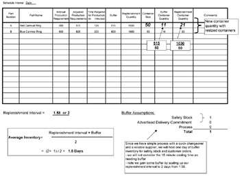
Figure 4-21: Corrected Kanban Quantities for Example 1.

Incorrect Production Data

Once you rule out containers as a culprit, determine whether you are using the correct production data. If you are using incorrect production requirements, you will either inflate or reduce the required run time. Check your current build plans and forecast. Have you used old data or artificially high requirements that drove up the production requirements? Also, review your scrap numbers for accuracy:

• Are the scrap quantities out of date?
• Has one scrap rate been applied in a broad brush when the different part numbers really have their own unique scrap rates?

Next , review your downtime data: Have you used real data or guessed? The downtime data will affect the time available for changeovers and can drive your replenishment interval to be negative. In the real world, a true negative replenishment interval means that you have a capacity problem. Therefore, when you calculate a negative replenishment interval, ask yourself: Am I running overtime or stocking out the customer?

The same issues apply to changeover data as for the scrap and downtime data. Are you using the real data or estimates? Did you use the same changeover times for all the parts when they are really different? Remember that since you are building a bank of time that allows you to cover all the changeovers, high changeover times result in higher replenishment intervals and higher inventories.

Incorrect Buffer Assumptions

The next item to consider is lead time. When assessing lead times ask these questions:

• Did you use the lead time you would like to have or what you really need?
• Do you really need all the contingencies you have planned for in the buffer inventory?

Take a good look at the buffer and make sure you are comfortable ”not extremely overweight!

Incorrect Capacity Assumptions

The last item to consider is the capacity issue. If you must produce on a six- or seven-day schedule to support your customer's fiveday schedule, then you must adjust the production requirements accordingly to account for this disconnect. Essentially, if your customer is on a daily schedule, then sum the weekly requirements and divide by six or seven to get your daily production requirements. Without scaling the requirements, you inflate the customer's requirements.

If you must produce on a six- or seven-day schedule to support your customer's five-day schedule, then make sure your buffer reflects this production disconnect. Your buffer must allow you to keep the customer supplied even though they will pull at a greater rate than you can replenish during their workweek. Finally, assess if this is a long- term situation to determine whether you need additional capacity to match your demand.

Reconciling the Problem

Take a systematic look at each of these factors to see why your calculated quantities do not parallel how you currently produce. Also, remember that the door swings both ways, so do not automatically accept your calculated kanban quantities being dramatically reduced. As a rule of thumb, review your numbers if the calculated quantities drop by more than 10 to 15 percent.

Once you have finalized the kanban quantities, then you and your team are ready to design the kanban's structure, which is the subject of Chapter 5. The rest of this chapter discusses an approach that does not utilize such in-depth calculations, looks at sizing supplier kanbans and at calculating the savings from implementing kanban scheduling.

An Alternate Method for Sizing Your Kanban

A second method, which yields results without as much data collection or calculations as the first method, is to make your current production schedule quantities the kanban quantities . This method does not lead to inventory reductions, but does have several advantages for organizations that want to move out quickly on kanban scheduling. The advantages of this method are that it:

• Reduces data collection requirements and implementation time, since you simply make your existing schedule quantity the kanban quantity
• Eliminates worries over incorrectly calculating the quantities, since you already know that the current schedule supports the production requirements

Although you do not engage in the same in-depth calculations as the first method, you should still follow the suggestions presented later in Chapter 9 when considering reductions in the kanban quantities. By following these suggestions, you ensure that you are not creating a problem that costs more than the savings. (Remember, there is no free lunch ”to reduce quantities some action must take place!)

For those organizations that have problems with following the schedule and are either underproducing or overproducing, you may find that this kanban will reduce your total inventory. The kanban can insert the necessary control if you design controls on containers and storage area. Figure 4-22 contains an example of this method using the data from Figure 4-10 (ten-part number) example.

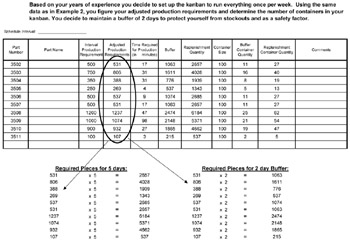
Figure 4-22: Example of the Alternate Method for Sizing Your Kanban.

Note that the quantities in Figure 4-22 differ from those calculated by Method 1 (shown in Figure 4-20). The increased quantities reflect the difference between this method versus the calculation method ”you have arbitrarily picked the kanban quantities and have not modeled the kanban after your system's capability. Therefore, you have not optimized the batch size ”you still have excess production in the system.

Supplier Kanbans

When extending kanbans to suppliers, you need to assess their ability to resupply your process. This assessment should include: shipment intervals, delivery time, quality issues, reliability issues, and demand fluctuation. In terms of calculating their replenishment interval ”don't bother. Don't dig into their data unless your initial discussions with the supplier on kanban quantities makes them want to add safety stock to your inventory. Otherwise, relay your requirements to them and let them accept the requirements.

Don't bully your suppliers into accepting your desired kanban plans ”it is a recipe for disaster. You must work with them to develop a plan that they can support. Once you have a mutual agreement on the kanban quantities, then follow the steps outlined in Chapter 5 to develop a mutually agreeable design to control the kanban between your operation and your supplier.

If you encounter resistance when dealing with suppliers on establishing kanbans, determine whether their resistance is based on lack of knowledge or unwillingness to change. If you value the supplier, then you should consider attempting to educate them on the benefits of kanban. On the other hand, their resistance may be a signal to consider changing suppliers.

Setting Up Supplier Kanban Quantities

To develop the kanban quantity, look at the delivery interval. This becomes the maximum replenishment quantity. In other terms, if you get a weekly delivery, then the replenishment interval must be one week. As you might suspect, this delivery interval may be an opportunity for improvement. To reduce the interval, you must look at your needs and the cost, then communicate these desires to your supplier. Once again, get the supplier to accept these new requirements, don't force them.

When considering a decrease in the delivery interval, which means receiving more frequent shipments, don't forget to consider transportation cost. You may end up decreasing inventory while dramatically increasing transportation cost. We will address some creative ways to reduce the delivery intervals in Chapter 9 when we discuss continuous improvement.

To determine your buffer for a supplier kanban, consider the delivery time, quality level, reliability level, and demand fluctuation. To handle the first three items, use your historical data on the supplier's performance. Also, determine whether the buffer created to cover the demand fluctuation will cover these items. As a rule of thumb, the kanban safety stock should not be greater than the current safety stock.

To handle demand fluctuation, consider your current order variation. To assess variation, calculate an average and standard deviation of your last ten orders or some other representative timeframe. (Once again we remind everyone not to be intimidated by the statistics terms and use the canned functions found in most spreadsheet programs.) Look at the standard deviation to determine how much the quantities vary over time.

If the demand fluctuation for the product is greater than 25 to 30 percent, then seriously reconsider the implementation of kanban and stick with forecasting. Additionally, in situations of extreme demand fluctuation, wait until you have successfully implemented several internal kanbans before taking it on.

If the standard deviation is 5 percent of the average or less, then don't worry about demand fluctuation. In this case, create a buffer to just cover delivery, quality, and reliability.

If the demand fluctuation exceeds 5 percent, then use a confidence interval to size the buffer. The confidence interval is a statistical factor that predicts the likelihood of an event occurring. We would suggest using the confidence intervals generated for a normal distribution. To use the confidence interval to size the buffer, simply multiply the standard deviation by the confidence interval. This quantity will become your safety stock. Typically, we recommend a confidence interval of 90 to 99 percent depending upon the impacts of stocking out.

To eliminate the phobia associated with the use of statistics by mere mortals , we have listed confidence intervals for 85 percent to 99 percent in Figure 4-23. Additionally, to further explain this concept, Figure 4-24 shows an example of a buffer based on various confidence factors.

Confidence Interval (based on a normal distribution)	Value
99%	2.326
97.5%	1.960
95%	1.645
92.5%	1.440
90%	1.282
87.5	1.150
85%	1.036

Figure 4-23: Confidence Intervals for Sizing the Kanban Buffer With Demand Fluctuation.

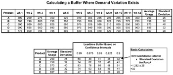
Figure 4-24: Calculating a Buffer Where Demand Fluctuation Exists.

Notice in the Figure 4-24 example how the buffer gets smaller as you decrease your confidence interval. Therein lies the heart of selecting safety stock confidence interval ”how much risk can you afford versus how much inventory do you want to hold?

From our experience it is best to perform a quick stock out analysis to see whether the calculated buffer would have supported the demand used to calculate the quantity. To perform this analysis:

• Subtract the demand quantity for each part number from the shipment (or average order) plus the calculated buffer.
• Repeat this operation for all the demand quantities used to calculate the average shipment and buffer.
• Now look at the results to see whether the on-hand quantity (shipment plus buffer) went negative or close to negative.

If the on-hand quantity goes negative, then reassess the confidence interval used to calculate the buffer and make changes as appropriate. Figure 4-25 shows an example of the proposed analysis using the data from the example in Figure 4-24. Notice how stock outs occur more frequently in the example as the confidence interval decreases.

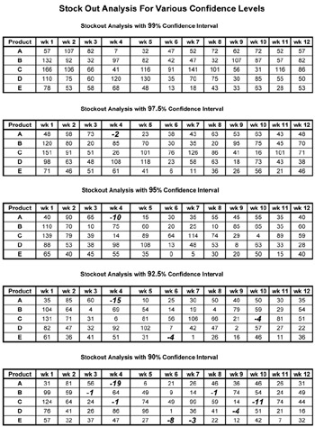
Figure 4-25: Stock-Out Analysis Using Figure 4-24 Data.

Finished Goods Kanbans

Follow the same advice for setting up finished goods kanbans as for the supplier kanban. Look at the customer demand and its fluctuation. However, in this case, you will need to assess your own delivery, quality, and reliability. Once you have that information, use the calculation method to calculate the kanban quantities .

If you have extreme demand fluctuation, again consider forecasting production versus kanban scheduling. Remember, two of your goals should be customer satisfaction and on-time deliveries that maintain customer satisfaction and manage cost.

Finally, follow the steps outlined in Chapter 5 on designing the controls for the kanban. Also, carefully consider any plans for making a finished goods kanban your first implementation project. You do not want to develop kanban implementation experience at the customer's expense.

Calculating the Benefits of Proposed Kanban

Once you have completed sizing the kanban, you may want to calculate the savings from implementing kanban. Typically, most senior managers will ask what the plant gains by implementing this system, so you need to be prepared to address the question. The kanban savings come from:

• Reduced inventory
• Reduced carrying cost
• Reduced space
• Reduced obsolescence cost

To calculate the savings, look first at the calculated inventory versus the current inventory to determine the inventory reduction. This inventory reduction translates into reduced inventory carrying cost. To calculate the reduced carrying cost, provide the inventory reduction information to your accountants and they can do the calculations.

The space reduction savings will be based on the other potential uses for the freed-up space. This savings will take the form of cost avoidance because the new construction or leased space will not be required. However, the identification of the space reduction may have to wait for the next phase and the design of the controls. Additionally, you can only assign a dollar savings to the space reductions if you have some other use for this space.

The reduced obsolescence cost will be a future cost avoidance rather than a hard cost. This figure will be based on history and the expectation of not making the same mistakes again.

One last item on calculating cost savings is how you should respond to the management question of: Can you reduce the inventory further without making process improvements? Remember that stock outs can also cost money and that stock outs become more likely as the inventory is reduced.

On the other hand, the cost of a stock out is determined by where the stock out occurs. If you have a safety stock of finished goods, then your customer is protected from minor supply disruptions from your internal and external suppliers. Thus the finished goods safety stock can allow you to be aggressive with internal kanban sizes while minimizing the risk of customer stock outs.

So before you get too aggressive, remember the downside. Remember that part of your plan should be to reduce quantities after you have the kanban operating successfully, so don't worry about being conservative in the early days of the kanban.

What About Economic Order Quantities vs the Calculated Kanban Quantity?

Many opponents of kanban like to discuss the need for economic order quantity (EOQ) calculations to determine whether the kanban quantities are correct. EOQ theories essentially attempt to calculate the batch size that minimizes the total cost. EOQ theory, however, does not consider the amount of inventory that can accumulate in the attempt to minimize the batch cost. EOQ supporters want to make these calculations to justify not doing kanban. Appendix E contains a detailed discussion of EOQ versus kanban and shows the benefits of kanban.

Regardless of the potential savings from using the EOQ model, you do not achieve the operational benefits of kanban scheduling without implementing kanban. Additionally, you have to store the inventory calculated by the EOQ model somewhere even if you have a lower batch cost. Therefore, when looking at the benefits of kanban, look beyond the raw dollar savings to the other benefits, such as flow, improved quality, empowerment of the operators, and space requirements.

Using the Workbook

The CD-ROM Workbook contains the kanban calculation form to help with the calculations for the kanban size . Use this form to calculate your kanban quantities . The workbook also contains the answers to the examples in Figures 4-9 and 4-10. Additionally, to facilitate the use of the equations, the Workbook and Figure 4-26 contain a summary of the equations presented in this chapter.

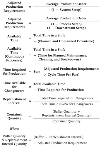
Figure 4-26: Summary of Equations for Using Method 1 to Calculate the Kanban Size.

Summary

In this chapter you learned how to calculate the kanban quantities for your process. We proposed two methods for determining the quantities :

1. Calculate the optimal kanban quantity based on your current process data.
2. Use the current schedule quantity to set up the kanban.

Both methods have decided benefits. Method 1 allows you to optimize the kanban quantities based on the current state of the process, which requires accurate data gathering to make sure you get true results. Figure 4-26 summarizes the equations for using this method, and Figure 4-27 ties these equations to the replenishment interval worksheet.

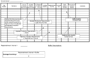
Figure 4-27: Application of the Forms to the Replenishment Interval Worksheets.

If the initial results do not look correct when using Method 1, then look at these areas for possible errors:

• Container sizes force added inventory
• Incorrect production data ”production requirements, scrap, downtime, and changeovers
• Incorrect buffer assumptions
• Incorrect capacity assumptions

Method 2 allows you to avoid the calculations and quickly determine the kanban quantities. However, this method maintains the potential excesses of the current schedule and achieves no calculated inventory reductions.

Regardless of which method you select, when reducing the kanban quantities, use the techniques presented in Chapter 9 to make the reductions. Remember that there is no free lunch , so don't arbitrarily reduce quantities. See Figures 4-14 through 4-17 for examples of how the continuous improvement process can dramatically affect the kanban quantities.

When you begin the process of implementing supplier kanbans, use demand data to develop the order quantity and buffer quantity. Follow the steps layed out in the chapter to calculate these quantities. Once you have these quantities, conduct a quick stockout analysis to confirm the appropriateness of the buffers.

When implementing supplier kanbans, make sure that the supplier agrees to your plans. To develop the kanban quantities, use the information in this chapter to determine the necessary buffers. We also propose use of confidence intervals to handle demand variation.

Use the same process proposed for the supplier kanban to size finished goods kanbans. Do not make a finished goods kanban your first project since learning kanban at the customer's expense may not be the wisest move.

When you have the kanban sized , look at the potential savings. Savings can come from inventory reductions, space reductions, carrying cost reductions, and elimination of obsolescence cost.

Review Appendix A if you have concerns about how EOQ compares to the proposed calculation process. Appendix E proposes an EOQ model and contrasts EOQ versus kanban. Regardless of the potential savings from using the EOQ model, you do not achieve the operational benefits of kanbans without implementing kanban. Additionally, you have to store the inventory calculated by the EOQ somewhere even if you have a lower batch cost.

Finally, the form in the CD-ROM Workbook will help you calculate the replenishment interval, buffer, and container quantities for your kanban.