3. Stochastic Dynamic Programming Approach

3. Stochastic Dynamic Programming Approach

In this section, we attempt to model the interactive VoD system using stochastic dynamic programming (DP). We model the arrival, departure and interactions in the systems as events, and as in a standard DP based approach, we apply an optimization "control" at the occurrence of each event. Let us consider the system at time t₀ = 0. Suppose there are N users u₁,u₂,…,u_N in the system (for simplicity of analysis we assume all users receive the same program) at that particular time instant, and their program positions are given by a sorted position vector P = (p_1, p₂,…, p_N), respectively, where p₁ ≥ p₂ ≥ ⋯ ≥ p_N . Because this is an aggregation based system, the number of streams in the system, n, is less than the number of users. Because the user position vector P is sorted, the stream position vector can be easily constructed from P in linear time. Therefore, the state of the system can be denoted in two ways: (1) by the user position vector P as described in the previous paragraph, or, (2) by a stream position vector S = (s₁,s₂,…,s_n) with ID's of users that each stream is carrying. We choose the latter representation for our analysis in this section.

In the following analysis, we assume that the N^th user arrived at time, t₀. Hence, p_N = 0, s_n = 0 and we must apply an optimization control at this time instant. An optimization control is nothing but a merging schedule which results in the minimization of the total number of streams in the long run under steady state. A merging schedule is a binary sequence M = (r₀,r₁,…,r_n) of length n, where r_i denotes the content progression rate of stream s_i, and r_i ∈ {r, r + Δr}, ∀i.

We describe a model for the events in the system. Suppose, the next event occurs at time instant t₀ + τ . The streams in the system progress according to the merging schedule M, which was prescribed at time t₀. The new position vector S' will be a function of the old position vector S, the merging schedule M, the inter-event time τ and also the type of event. The size of the position vector S, increases, decreases or stays the same depending on the type of the event:

• Arrival: size increases by 1

• Departure due to a user initiated quit: size decreases by 1 (if the quit is initiated in a single-user stream) or stays the same (if the quit is initiated in a multi-user stream)

• Exit due to the end of the program: size reduces by 1, and number of users on the exiting stream.

• Interaction: size increases by 1 (if initiated in a multi-user stream) or stays the same (if initiated in a single-user stream)

3.1 Cost Formulation for Stochastic Dynamic Programming

We begin with a brief introduction to the stochastic DP approach [5] that we decided to utilize to model the system. The quantity that we want to minimize in the system is the number of streams, n, in steady state. Using the DP terminology, we refer to this quantity as average cost incurred per unit time. The total average cost incurred can be represented by a sum of short-term cost and long-term cost per unit time. The former reflects the immediate gains achieved by the merging schedule M (i.e., before the next event occurs), whereas the latter reflects the long term gains due to M. If the current state (basically the position vector S at time t₀) is represented by i and the long-run cost incurred at state i is denoted by a function h(i), then the total average cost per unit time at the current time instant t₀ is given by the Bellman's DP equation:

(37.12)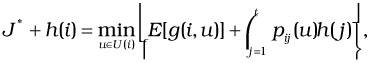

where U(i) is the set of possible controls (merging schedules, in our setting) that can be applied in state i, g(i, u) is the short-term cost incurred due to the application of control u in state i, E[g] denotes the expected value of the short-term cost, p_ij(u) denotes the transition probabilities from state i to state j under control u and h(j) is the long-run average cost at state j. t is a state that can be reached from all initial states and under all policies with a positive probability, and J* is the optimal average cost per unit time starting from state t.

The Curse of Dimensionality

Under this formulation, we quickly run into some problems. First, the state space is very large. If the maximum number of users in the system is N and the program contains L distinct program positions, the number of states is clearly exponential in N, no matter how coarsely the program positions are represented (obviously, this depends on the coarseness of representation). For fine grain state representations, the size of the state space grows exponentially as well. Also, the space of controls is exponential in n, where n denotes the number of streams in the system, because each stream has two choices for the content progression rate. Furthermore, the long-run cost function h( ) is very hard to characterize for all states especially in the absence of a formula based technique. Currently we believe that h( ) can be characterized by running a simulation for long enough that states start to recur and then the long run average cost values can be updated for every state over a period of time. However, this technique is extremely cumbersome and impractical owing to the hugeness of the state space in a VoD system with a large dimension (N). Therefore, due to this curse of dimensionality, we believe that the DP method is impractical in its actual form and attempt to use it in a partial manner, which we explain in detail next.

Expected Cost Calculation

Figure 37.6 demonstrates the basic model of events and controls. The left side depicts the occurrence of events e and e + 1 for a section of the timeline. The inter-event time is τ and the system moves from state i to state j under control u and incurs a short-term expected cost denoted by E[g(i, u)] which depends on the distribution of the random variable τ. We illustrate a technique for the calculation of this quantity below.

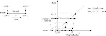
Figure 37.6: Event model and controls.

The control space is chosen carefully to prevent an exponential search and to yield an optimal substructure within a control. u is considered to be a feasible control if it represents a binary tree with s₁, s₂,…,s_n as leaves. Hence u is a function of the state i. Although the control space U(i) grows combinatorially with n, the use of the principle of optimality (as demonstrated later) results in a polynomial time algorithm for choosing the optimal control. On the right side of Figure 37.6, a control is shown as a binary tree which is a function of state i. We depict the intermediate merge points in the binary tree by t_k:1 ≤ k ≤ n - 1; t₁ ≤ t₂ ≤ ⋯ ≤ t_n-1. denotes the time that the leading stream will run. Here we assume that the leading stream goes fast after the final merge and that all n streams merge before the movie ends (i.e., . t_k 's can be determined easily from the stream position vector (essentially state i) and the control under consideration, u.

We formulate the short-term cost function for a given state i and a control u as the cost per unit time between events e and e+ 1. For simplicity, we assume that t₀ = 0; because this contributes to an additive term in the expected cost formulation and it does not affect the comparison of costs under two different controls.

(37.13)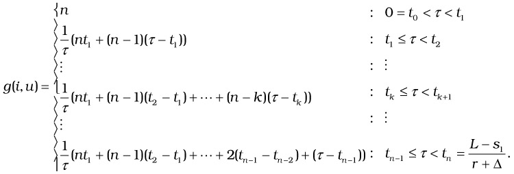

The general (k^th) branch in the above cost formulation simplifies to the following:

(37.14)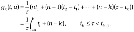

The only random variable in the above analysis is the inter-event time τ which is exponentially distributed because the occurrence of various events can be modeled by the Poisson distribution. In particular, if the arrivals occur with a mean rate λ_a, quits occur with a mean rate λ_q, and interactions occur with a mean rate λ_i, and each is modeled by the Poisson distribution, then the aggregate event process is also Poisson with a rate λ = λ_a + λ_q + λ_i (i.e., the mean inter-event times (τ) are exponentially distributed with mean λ). The expected cost under control u can be calculated in the following manner.

(37.15)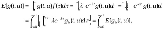

where E[g_k(i, u)] is given by

(37.16)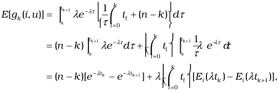

where . From Equation 37.15, after algebraic simplification, we yield a compact expression for the expected cost:

(37.17)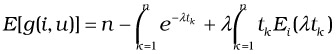

Stochastic RSMA

Having derived an expression for the expected short-term cost, we attempted to use it for choosing the optimal control. In other words, given that we are in state i, we find the control u(i) that minimizes E[g(i, u(i))]. Instead of direct constrained minimization, we use the principle of optimality and the separability of terms in Equation 37.17 to represent the cost recursively as follows.

(37.18)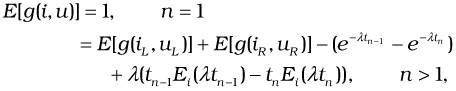

where u_L and u_R represent the left and the right subtrees of u, respectively, and i_L and i_R represent the corresponding portions of the state i. Because t_n-1 is fixed for a given state i, a static DP approach that is very similar to the RSMA-slide approach described in Section 2 can be applied to produce the optimal u. The time complexity of this algorithm, called Stochastic RSMA, is O(n³). Simulation results for the algorithm are shown in Section 4.6.