2. Stream Clustering Problems

2. Stream Clustering Problems

Here we characterize the space of on-demand video stream clustering problems by formulating a series of sub-problems. We provide optimal solutions for some of these sub-problems and present heuristic solutions derived from these optimal approaches for the remainder.

2.1 General Problem Description

A centralized video-server stores a set of k movies M = {M₁,M₂,…,M_k}, each having lengths l₁,l₂,…,l_k, respectively. It accepts requests from a pool of subscribers for a subset of these stored movies and disseminates the content to the customers over a delivery network which supports group communication (e.g., multicast). Assume that the movie popularity distribution is skewed (non-uniform) obeying a probability distribution P( ). Each popular movie can be played at two different content progression rates, r (normal speed) and r + Δr (accelerated speed). Accelerated versions of these movies are created by discarding some of the less important video frames (e.g., B frames in the MPEG data stream) by the server on the fly. If the frame dropping rate is maintained below a level of ≈ 7%, the minor degradation of quality is not readily perceivable by the viewer [4,16].

There is an opportunity to reclaim streaming data bandwidth if skewed streams of identical movies are re-aligned and consolidated into a single stream. This can be achieved by the server attempting to change the rate of content progression (the playout rate) of one or both of the streams.

There are several means of delivering the same content to a group of users using a single channel. Multicast is a major vehicle for achieving this over the IP networks. But because it has not been widely deployed in the general Internet, another scheme called IP Simulcast can be used to achieve the same goal by relaying or repeating the streams along a multicast tree [9]. If the medium has broadcasting capabilities (such as cable TV channels) multicast groups can be realized by means of restricted broadcast.

The term clustering refers to the action of creating a schedule for merging a set of skewed identical-content streams into one. The schedule consists of content progression directives for each stream at specific time instants in the future. For large sets of streams, the task of generating this schedule is computationally complex and is exacerbated by the dynamics of user interactions to achieve VCR functions such as stop, rewind, fast-forward and quit. It is clear that efficient algorithms for performing this clustering are needed for large sets of streams. The term merging refers to the actual process of following the clustering algorithm to achieve the goal.

A general scenario for aggregation of video streams with clustering is outlined below. At time instants T_i the server captures a snapshot of the stream positions - the relative skew between streams of identical content - and tries to calculate a clustering schedule using a clustering algorithm CA for aggregating the existing streams. Aggregation is achieved by accelerating a trailing stream towards a leading one and then merging whenever possible. Changing the rates of the streams is assumed to be of zero cost and the merging of two streams is assumed to be seamless. Viewers, however, are free to interact via VCR functions and cause breakouts of the existing streams. That is, new streams usually need to be created to track the content streaming required for the VCR function. Sometimes these breakouts are clusters themselves when more than one viewer initiates an identical breakout. The interacting customers are allocated individual streams, if available, during their interaction phase but are attempted to be aggregated at the next snapshot epoch. We restrict our discussion to the VCR actions of fast-forward, rewind, pause, quit.

Figure 37.1 illustrates the merging process. Here the lifespans of several streams receiving the same content are plotted over time. The horizontal axis denotes the position of a stream in the program and the vertical axis is the time line. The length of the movie is assumed to be L as indicated by the vertical line on the right. Streams are shown in one of the following three states: normal playback, accelerated or paused. Accelerated streams have a steeper slope than the normal streams because they move faster than the latter. Paused streams have infinite slope because they do not change their position with time. Between time 0 and T₁ all arriving streams progress at a normal rate.

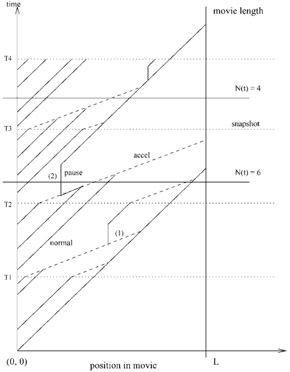
Figure 37.1: Aggregation of streams.

The first snapshot capturing positions of existing streams occurs at time T₁. At this time a clustering algorithm is used to identify the clusters of streams that should be merged into a single stream (per cluster). The merging schedule is also computed within each cluster. Different algorithms can be applied for performing the clustering and merging (see Section 4). When new users arrive in between snapshots they are advanced at a normal rate until the next snapshot when the merging schedule is computed again and the streams are advanced according to the new clustering schedule. The clusters and the merging schedule are computed under an assumption that no interactions will occur before all the streams merge. But because the system is interactive, users can interact in the middle. If a user interacts, on a stream that is carrying multiple users, a new stream is allocated while the others on the stream continue. Case (1) in the figure demonstrates this phenomenon. However, if the only user on a stream interacts, the server stops sending data on the previous stream because it does not carry any user anymore. This is illustrated by case (2) in the figure. N(t) denotes the number of streams existing in the system at a time instant t.

A state of a non-interacting stream S_i can be represented by a position-rate tuple (p_i, r_i), where p_i ∈ ℜ⁺ is the program position of the i^th stream, measured in seconds from the beginning of the movie and r_i ∈ {r, r + Δr} is the content progression rate. The state equation is given by:

(37.1)

and r_i(t) is determined by the clustering algorithm CA. Note that in this discussion, time is measured in continuous units for simplicity. In reality, time is discrete as the smallest unit of time is that required for the play-out of one video frame (approximately 33 ms for NTSC-encoded video).

As an example of a merge, consider streams S_i (rate r) and S_j (rate r + Δr). If they can merge in time t, then the following will hold:

(37.2)

(37.3)

The most general problem is to find an algorithm CA that minimizes , the average number of streams (aggregated or non-aggregated) in the system in a time interval [ττ + T] for given arrival and user interaction rates. The space of optimization problems in this aggregation context is explored next.

2.2 Clustering Under a Time Constraint

There is a streaming bandwidth overload scenario that exists when too many users need unique streams from a video server. This scenario arises when many users interact simultaneously, but distinctly, or when a portion of a video server cluster fails or is taken offline. The objective of a solution for this scenario is to recover the maximum number of channels possible within a finite time budget, by clustering outstanding streams. We assume that interactions are not honored during the recovery period because the system is already under overload.

Maximizing the number of channels recovered is desirable because it enables us to restore service to more customers and possibly to admit new requests. Recovery within a short period of time is necessary since customers will not wait indefinitely on failure. It is possible to mask failures for a short period of time by delivering secondary content such as advertisements [17]. This period can be exploited to reconfigure additional resources. However reconfigurability adds substantially to system costs and additional resources may not be available.

Optimal stream clustering under failure can be solved easily in polynomial time and a linear-time algorithm using either content insertion or rate adaptive merging is described in reference [16]. This algorithm, called EMCL (Earliest Maximal CLuster), starts from the leading stream and clusters together all streams within the time budget, then repeats the process by starting from the next stream ahead until the final, trailing stream is reached. A more general class of one-dimensional clustering problems has been shown to be polynomially solvable [12].

Three points are worth noting here. Firstly, the EMCL algorithm can be applied when both content insertion and rate adaptation are used. The number of channels recovered by the algorithm is non-decreasing with increase in the time budget. Using both techniques has the same effect as increasing the time budget when using one technique alone. Therefore we can apply the same algorithm. We will see later that this property does not generalize to other optimization criteria.

Secondly, this algorithm is not affected if some leading streams will reach the end of the movie before clustering. By accelerating all streams that are within the time budget from the end of the program and then computing the clustering for the remaining streams, we can achieve an optimal clustering.

Thirdly, iterative application of this algorithm does not provide further gains in the absence of interactions, exits or new arrivals. In the dynamic case, the average bandwidth, in number of channels, used during clustering is of consequence. We consider this average bandwidth minimizing constraint and dynamicity in the following sections.

2.3 Clustering to Minimize Bandwidth

Another goal for clustering is to minimize the average bandwidth required in the provisioning of a system. This can be measured by the number of channels per subscriber and is more interesting and applicable from a service aggregation perspective. A special case of this problem occurs when we wish to construct a merging schedule at some instant that uses minimum bandwidth to merge all streams into one to carry a group of users. Ignoring arrivals, exits and breakaways due to interaction, the problem has been approached heuristically by Lau et al. [18] and analytically by Basu et al. [3].

The problem can be readily transformed into a special case of the Rectilinear Steiner Minimal Arborescence (RSMA) problem [3], which is defined by Rao et al. [19] as:

Given a set N of n nodes lying in the first quadrant of E², find a minimum length directed tree (called Rectilinear Steiner Minimal Arborescence, or RSMA) rooted at the origin and containing all nodes in N, composed solely of horizontal and vertical arcs oriented from left to right and from bottom to top.

The transformation is illustrated in Figure 37.2 with a minor difference that an up arborescence - a directed tree with arcs directed towards the root - is used instead. In the figure on the left, the shaded dots denote the stream positions at the time instant corresponding to the beginning of the snapshot. Each stream has a choice of either progressing at a normal speed (larger slope in the figure) or at an accelerated speed (smaller slope). In the optimal tree, the absolute trailer must always be accelerated and the absolute leader must always be retarded, and the two lines corresponding to them will meet at the root. In Steiner tree terminology the shaded dots (∈ N) are called sinks. The RSMA is denoted in the figure on the right as a rooted directed tree (the arrow directions have been reversed for a better intuitive feel).

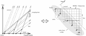
Figure 37.2: Minimum bandwidth clustering.

In the RSMA formulation, normal streams move horizontally whereas the accelerated streams move vertically. The leader always remains horizontal and the trailer vertical. The sinks lie on a straight line of slope =-1 and the final merge point which is the root of the RSMA is at the origin. This transformation leads to a special case of the RSMA problem in which the sinks form a slide. The slide is a configuration without a directed path from one sink to another (i.e., there are no sinks in the interior of the rectilinear grid (called a Hanan grid). Note that this special case of the problem has an optimal sub-structure that is lacking in the general case, and finding the min-cost RSMA spanning n sinks is equivalent to finding an optimal cost binary tree on n leaf-nodes or an optimal bracketing sequence. The number of binary trees on n leaf-nodes (or RSMAs with n sinks forming a slide) is given by the (n - 1)^st Catalan number, . Although this constitutes an exponential search space, the special structure of the problem allows us to compute an optimal binary tree using a dynamic programming (DP) algorithm of complexity O(n³) [19]. One can easily verify that the RSMA for the particular placement of sinks in Figure 37.2 is a minimum length binary tree. We call the DP algorithm RSMA-slide in this chapter.

One point to be noted here is that from an optimality standpoint, more than two content progression rates are not needed. Figure 37.3 illustrates the situation. A line segment with a higher Cartesian slope has a higher content progression rate. In Figure 37.3(a), three rates are used for content progression and the streams yield a single meeting point. Clearly the merging trees in Figures 3(b-c) have lower cost in terms of bandwidth used than the previous one, because a merge occurs earlier in those two cases. Therefore, two content progression rates are sufficient for rate adaptation.

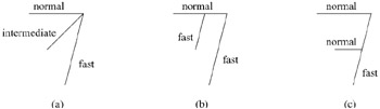
Figure 37.3: Merging with more than two rates.

Now, we describe the RSMA-slide algorithm which is based on optimal binary trees [2]. Let L be the length of the movie that is served to streams i,…, j , with p_i > p_j . P(i, j) denotes the optimal program position where streams i and j would merge and is given by:

(37.4)

(37.5)

Let T(i,j) denote an optimal binary tree for merging streams i,…,j. Let Cost(i, j) denote the cost of this tree. Because this is a binary tree, there exists a point k such that the right subtree contains the nodes i,…,k and the left subtree contains the nodes k + 1,…,j . From the principle of optimality, if T(i, j) is optimal (has minimum cost) then both the left and right subtrees must be optimal. That is, the right and left subtrees of T(i,j) must be T(i,k) and T(k + 1, j). The cost of this tree is given by

(37.6)

(37.7)

and the optimal policy merges T(i, k*) and T(k* + 1, j) into T(i, j), where k* is given by

(37.8)

Here Cost(i, k) and Cost(k + 1, j) are the costs of the right and the left subtrees respectively, calculated until the end of the movie.

We begin by calculating T(i, i) and Cost(i, i) for all i. Then, we calculate T(i, i + 1) and Cost(i, i + 1), then T(i, i + 2) and Cost(i, i + 2) and so on, until we find T(1, n) and Cost(1, n). This gives us our optimal cost. The algorithm can be summarized as follows:

Algorithm RSMA-slide

 {    for ( i = 1 to n )       Initialize P(i, i), Cost(i, i) and T(i, i) from eqns. 4 and 6    for (p = 1 to n - 1)      for (q = 1 to n - p)        Compute P(q,q + p), Cost(q,q + p) and T(q,q + p) from eqns. 5, 7 and 8 } 

There are O(n) iterations of the outer loop and O(n) iterations of the inner loop. Additionally, determination of Cost(i, j) requires O(n) comparisons in the argmin step. Hence, the algorithm RSMA_Slide has a complexity of O(n³). Therefore, we conclude that the static clustering problem has an optimal polynomial time solution, in contrast to the conclusion of Lau et al. [18]. Note that in practice, n is not likely to be very high, thus making the complexity acceptable.

Although optimal binary trees are a direct way to model this particular problem (where there are no interactions), the RSMA formulation offers more generality as we shall explain in later sections. Recently, Shi et al. proved that the min-cost RSMA problem is NP-Complete [21]. However, before RSMA was proved to be NP-Complete, Rao et al. had proposed a 2-approximation algorithm of time complexity O(n log n) for solving the RSMA [19].

Minimum bandwidth clustering can be used as a sub-scheme to clustering under a time budget, so that channels are released quickly thereby accommodating some interactivity. This technique can speed up computations in a dynamic scenario, in which cluster re-computation is performed on periodic snapshots. The time-constrained clustering algorithm has linear complexity and the dynamic programming algorithm of cubic complexity needs to be run on a smaller number of streams. Simulation results for these are shown in Section 4.

2.4 Clustering with Arrivals

Relaxing the preceding problem to include stream arrivals, but not exits nor other interactions, we consider continuing the investigation of the problem space. Suppose we could have a perfect prediction of new stream arrivals. The problem again transforms to the RSMA-slide formulation. Although the sinks do not lie on a straight line, they would still form a slide (e.g., the two points at the bottom right corner of Figure 37.4 form a slide along with the points lying towards their left in the exterior of the grid). Therefore, a variant of the RSMA-slide algorithm of Section 2.3 can be used here. The cost calculation can differ in this case because two points can merge by following paths of unequal length. For example, the two predicted points in Figure 37.4(b) are merged by line segments of different lengths. After the RSMA is calculated, a corresponding merging tree can be found for the original formulation as shown in Figure 37.4(a).

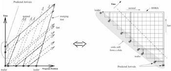
Figure 37.4: Clustering with predicted arrivals.

Alternatively, we can batch streams for a period equal to or greater than the maximum window for merging. In other words, the users that have newly arrived can be made to wait for an interval of time for which the previously arrived streams are being merged. Although this can reduce the problem to the preceding one, in practice, this can lead to loss of revenue from customer reneging due to excessive waiting times.

Aggarwal et al. [2] instead use a periodic re-computation approach with an initial greedy merging strategy. They show that if the arrival rate is fairly constant, a good re-computation interval can be determined. If a perfect predictor were available (e.g., via advance reservations), then better performance can be achieved by using the exact RSMA-slide algorithm.

2.5 Clustering with Interactions and Exits

Here we show how a highly restricted version of the problem with certain unrealistic assumptions is transformable to the general RSMA problem. We assume a jump-type interaction model (i.e., a user knows where to fast forward or rewind to, and resumes instantaneously). We also assume that the leading stream does not exit and that interactions do not occur in singleton streams (which are alone in their clusters). Furthermore we assume that a perfect prediction oracle exists which predicts the exact jump interactions. Our "perfect predictor" identifies the time and the program position of all user interactions and their points of resumption.

Figure 37.5 shows a transformation to the RSMA problem in the general case. The shaded points in the interior of the grid depict predicted interactions. The problem here is to find a schedule that merges all streams taking into account all the predicted interactions and consumes minimum bandwidth during the process. This problem is isomorphic to the RSMA problem, which has recently been shown to be NP-Complete [21]. Also, the illustration shows that the RSMA is no longer a binary tree in this case.

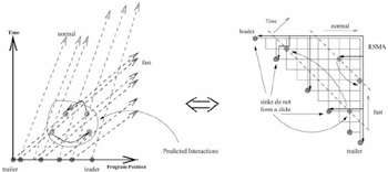
Figure 37.5: Clustering under perfect prediction.

Stream exits can occur due to the ending of a movie or a user quitting from a channel which has only one associated user. Exits and interactions by a user, alone on a stream, result in truncation and deletion of streams, respectively, and cause the RSMA tree to be disconnected and form a forest of trees. The above model is not powerful enough to capture these scenarios. Perhaps a generalized RSMA forest can be used to model these situations. However, the RSMA forest problem is expected to be at least as hard as the RSMA problem.

An approximation algorithm for RSMA that performs within twice the optimal is available using a "plane sweep" technique. But in a practical situation in which a perfect prediction oracle does not exist, knowing the arrivals, and especially interactions, beforehand is not feasible. Therefore the practical solution is to periodically capture snapshots of the system and base clustering on these snapshots. The source of sub-optimality here is due to the possibility that a stream could keep on following its path as specified by the algorithm at the previous snapshot even though a stream with which it was supposed to merge has interacted and does not exist nearby anymore. Only at the next snapshot does the situation get clarified as the merging schedule is computed again. Also note that causal event-driven cluster recomputation will perform worse than the perfect oracle-based solution. For any stochastic solution to be optimal and computationally tractable, the RSMA must be solvable by a low order polynomial time algorithm. The important point here is that because we do not have a low cost predictive solution in interactive situations, we must recompute the merging schedules periodically to remain close to the optimal.

Note that an algorithm with time complexity O(n³) (for RSMA-slide) may be expensive for an on-line algorithm and it is worthwhile comparing it with its approximation algorithm that runs faster, producing worst-case results with cost within twice the optimal. In the simulations section (Section 4), we compare both the algorithms under dynamic situations. Rao et al. [19] give a polynomial-time approximation algorithm based on a plane-sweep technique which computes an RSMA with cost within twice the optimal. The algorithm is outlined below.

If the problem is set in the first quadrant of E² and the root of the RSA is at the origin, then for points p and q belonging to the set of points on the rectilinear grid of horizontal and vertical lines passing through all the sinks, the parent node of points p and q is defined as parent(p, q) = (min(p.x, q.x), min(p.y, q.y)), and the rectilinear norm of a point p = (x, y) is defined by ||(x, y)|| = x + y.

Algorithm RSMA- heuristic( S :sorted stream list)

 {   Place the points in S on the RSA grid   while (S ≠ φ)    Find 2 nodes p, q ∈ S such that || parent(p,q) || is maximum    S ← -S {p,⋃ q) parent(p,q)    Append branches parent(p,q) → p and parent(p,q) → q to the RSA tree.  end } 

The algorithm yields an heuristic tree upon termination. Because it is possible to store the points in a heap data structure, we can find the parent of p and q with the maximum norm in O(log n) time and hence the total time complexity is O(n log n).

The fact that the static framework breaks down in the dynamic scenario is not surprising. Wegner [25] suggests that interaction is more powerful than algorithms and such scenarios may be difficult to model using an algorithmic framework.

2.6 Clustering with Harder Constraints and Heuristics

In practice, stream clustering in VoD would entail additional constraints. We list a few of them here:

• Limits on total duration of rate adaptation per customer

• Critical program sections during which rate adaptation is prohibited

• Limited frequency of rate changes per customer

• Continuous rather than "jump" interactions

• Multiple classes of customers with varying pricing policies

The inherent complexity of computing the optimal clustering under dynamicity, made even harder by these additional constraints, warrants search for efficient heuristic and approximation approaches. We describe a number of heuristic approaches which are worthy of experimental evaluation. We evaluate these approaches experimentally in Section 4.6.

• Periodic Periodically take a snapshot of the system and compute the clustering. The period is a fixed system parameter determined by experimentation. Different heuristics can be used for the clustering computation:

  15. Recompute RSMA-slide (optimal binary tree) using O(n³) dynamic programming algorithm.

  16. Use the O(n log n) RSMA heuristic algorithm.

  17. Use the O(n) EMCL algorithm to release the maximum number of channels possible.

  18. Follow EMCL algorithm by RSMA-slide, heuristic RSMA-slide or all merge with leader.

• Event-triggered Take a snapshot of the system whenever the number of new events (arrivals or interactions) exceeds a given threshold. In the extreme case, recomputation can be performed at the occurrence of every event.

• Predictive Predict arrivals and interactions based on observed behavior. Compute the RSMA based on predictions.

2.7 Dependence of Merging Gains on Recomputation Interval

In this section, we use analytical techniques to investigate the channel usage due to RSMA in the steady state. The modeling approach is more completely described in reference [15].

First, we derive an approximate expression for the number of streams needed to support users watching the same movie in a periodic snapshot RSMA-based aggregation system as a function of time. We consider the non-interactive case here. In a typical recomputation interval R, new streams arrive (one user per stream) at a rate λa; the older streams are included in the previous snapshot captured at the beginning of the current recomputation interval, and are merged using RSMA. Now, to make the calculation tractable, we assume that the process of capturing snapshots enforces a "natural clustering" of streams in the sense that the streams being merged in the current recomputation interval are less likely to merge with streams in the previous recomputation interval, at least for large values of R. This assumption is reasonable because the last stream of the current cluster (the trailer) accelerates while the leading stream of the previous cluster (leader) progresses normally, thus resulting in a widening gap between end-points of clusters.

We model one recomputation interval R, and then consider the effect of a sequence of R's by a summation. Again, we make a very simplistic assumption to make the problem tractable. We assume that the streams in a snapshot are equally spaced and the separation is . In this situation, the RSMA is equivalent to progressively merging streams in a pair wise fashion. If L is the length of the movie and K = 15 is a factor arising due to the speed-up, the number of streams as a function of time from the beginning of the snapshot is given by:

(37.9)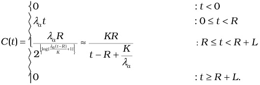

At any time instant t, the total number of streams N(t) is built from contributions of a sequence of recomputation intervals. It is given by:

(37.10)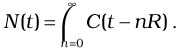

Note that only some of the terms in the above summation have a nonzero contribution to the total sum. We are interested in calculating the average number of streams in steady state, in other words, in the value of . But, it can be shown that N(t) is periodic with period R, hence we calculate the value of , where t₀ signifies a time instant after steady state has been reached.

As we indicated before, N(t) is non-zero only for a sequence of recomputation intervals; hence by appropriately taking contributions from relevant intervals, we get an expression for the average number of streams in the system in steady state:

(37.11)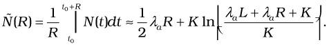

We observe that has a linear component in R and a logarithmic (sub-linear) component in R, thus making the overall effect linear in R, especially for large value of R. We shall see in Section 4.6 that this agrees in behavior with the simulation results, although there are inaccuracies in the exact values of N(t) due to the approximate nature of the model developed here.