9.4 Timed Petri nets
|
| < Free Open Study > |
|
9.4 Timed Petri nets
The Petri nets covered in the previous section had transitions that when fired took no time to move tokens from one place to another. In any real system an activity does take some finite time to perform its operation. For example, to read a file from a disk, to execute a program, or to communicate with some other machine takes some real time. Adding time to the Petri net provides the Petri net modeler with another powerful tool with which to study the performance of computer systems. Time can be associated with transitions, with selection of paths, with waiting in places, with inhibitors, and with any other component of the Petri net.
The most typical way that time is used in Petri net modeling is associated with transitions. This is because the firing of a transition can be viewed as the execution of an event being modeled-for example, a CPU execution cycle. Transitions that have time associated with them are referred to as timed transitions. These timed transitions are represented graphically as a rectangle or thick bars and are identified by designations beginning with t.
In Figure 9.23, transition t1 is a timed transition with time t1 as its interval to complete its firing once enabled. The semantics of the firing are a bit different from that of the basic Petri nets looked at previously. When a transition becomes enabled, its time period clock timer is set and begins to count down. Once the timer reaches 0, the transition fires, moving the token(s) from the input places for the transition to the output places for this transition. In the example shown in Figure 9.23, when a token arrives at place p1, the timer for transition t1 is set to τ1 and begins to count down. Once τ1 time units have passed, the transition fires and the token is taken from p1 and moved to p2. The decrement of the timer must be at a constant fixed speed for all transitions in the Petri net model. In this way the transition is made to model the operation of some element within the system being modeled.
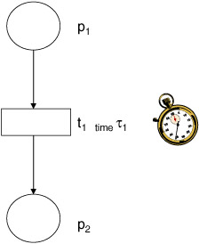
Figure 9.23: Timed Petri net.
A consideration to think about is what occurs when a transition becomes nonenabled due to the initial enabling token being used to ultimately fire a competing transition. This condition is shown in Figure 9.24. If we assume that the time for transition t1 is less than that for transition t2, then, when place p1 receives a token, the two timers would begin counting down. At some time (τ1) in the future, the timer for t1 would reach its zero value, resulting in the firing of transition t1. Since the token enabling t2 is now gone, t2 is no longer enabled and, therefore, its timer (τ2) would stop ticking down. The question now is what to do with transition t2's timer. There are two possibilities. The first is to simply reset the timer on the next cycle in which place p1 has a token present, enabling t2. In this case, unless place p1 has a state where it has more than one token present, transition t2 will never fire. The second possible way to handle this situation is to allow transition t2's timer to maintain the present clock timer value (τ2 - τ1). In this second case, when the next token is received at place p1, the timer for transition t1 resets its clock timer to τ1, and transition t2 will continue counting down from time (τ2 - τ1). If the remaining time in transition t2's timer is less than transition t's timer, then transition t2 will fire, leaving transition t1 with the remaining time (τ1 - (τ2 - τ1)). The choice of which protocol to use will depend on the system one wishes to model.
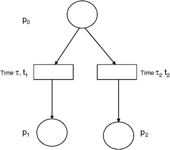
Figure 9.24: Timed Petri net with conflict.
The timing need not be exclusively based on timers and counting. Some Petri net models have proposed using state transition timing graphs. In this case, each possible state, μ, is enumerated, and a time period is set for each individual state to traverse from this state to the next state in the sequence (Figure 9.25). In this figure, state μ1 will require (τ2 or τ1) time units to move from state μ1 to state μ2 and so on for all states defined in our system. This could also be represented using timed transition sequences, which depict the order of each transition in relation to all others. Such a description may appear as:
| (9.7) |
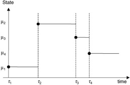
Figure 9.25: State transition timing graph.
Transitions can also be represented as immediate transitions-that is, transitions without any time delays associated with them. To model these in timed Petri nets, we simply can use a solid bar in the graphical mode or a timer of 0 if we are using Petri net notation.
In the example shown in Figure 9.26, we use immediate transitions to capture a resource. These act like semaphores would in a real system. One active process that is vying for the resource will win it, while the other will be forced to wait until the resource becomes free once again.
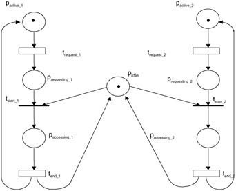
Figure 9.26: Timed Petri net with immediate transitions.
|
| < Free Open Study > |
|
EAN: 2147483647
Pages: 136