9.5 Priority-based Petri nets

---

9.5 Priority-based Petri nets

The Petri nets defined in the previous section were improvements over the basic nets defined in the first section of this chapter. To continue this trend we next look at adding priority to a Petri net. The formal model now needs some additional elements. The Petri net is described by a nine tuple, M = (P, T, I, O, H, ∏, Par, Pred, μ). P represents the set of places of Petri net M. T is the set of transitions of Petri net M. I represents the set of input functions for the transitions of M. O represents the set of output functions for the transitions of M. H represents the inhibitor functions defined over the set of transitions in M. Par represents the parameter set for this Petri net, and Pred represents the predicates defining how the parameter set can be distributed. The symbol μ represents the set of markings for this Petri net, and Π represents the priority function defined over all transitions of Petri net M. The function Π maps the priority for each transition to a set of integer values representing their importance relative to each other in the net.

Now we will look at the conditions for firing under these new nets. Transitions in priority Petri nets are enabled just as in basic Petri nets. If the transitions have their input places with the right amount of tokens, then they are prepared for enabling. The term used for this is concession. If a transition has concession (is enabled as in basic nets) and there are no additional transitions in this network that are enabled in the present marking with priority greater than this transition's priority, then it is enabled. Formally this set of conditions is represented as:

(9.8) 

A transition that meets these criteria can fire. The result of firing is the same as in nets without priority. In the example depicted in Figure 9.27, transition t₁ has the lowest priority at 1, transition t₂ has the next lowest at 2, and transitions t₃ and t₄ have the highest priority at 3. If we start with an initial marking, μ = (1,0,0,1), only transition t₂ is enabled, since it has the highest priority and has the number of tokens available from its input functions as required for enabling. If you compute the next few possible states, you would see that transition t₁ will never be enabled, since it does not have the priority to overcome transition t₂'s priority.

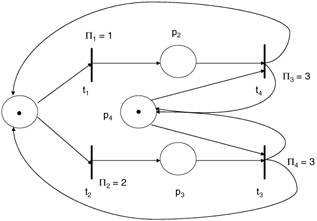
Figure 9.27: Priority-based Petri net.

With the use of priority and timing we can do a more complete job of defining conditions such as contention, confusion, and concurrency. For example, the Petri net shown in Figure 9.28 has both timed and priority features. By combining these features we can now get the system to toggle between the two events. The inhibitor on transition t₂ causes this immediate transition to be blocked from enabling until it has completed its service. In this way it allows transition t₁, with the lower priority, to get service while place p₂ has tokens present.

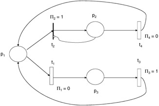
Figure 9.28: Timed and priority net.

---