7.2 Networks of queues

---

7.2 Networks of queues

Until now, we have been considering queuing systems that contain only one station. That is, the systems that we have looked at have a single queue and a single server or set of servers, and customers arrive only at that queue and depart only following service. This situation is fine for relatively simple systems that are either not connected to other systems or that can be considered isolated from other, connected systems. Now, we will consider the case in which several queuing systems are interconnected and attempt to find meaningful statistics on such a system's behavior.

Referring to section 7.1, we recall that a network of queues results from connecting the departure stream of one queuing system to the queue input of another, for an arbitrary number of queuing systems connected in an arbitrary way. Also, we discussed the concept of open and closed networks in which an open network was defined as one in which arrivals from, and departures to, the outside world are permitted, and a closed network is one in which they are not permitted. We will discuss general classes of both types here.

7.2.1 Closed networks

Consider the closed three-stage network of queues shown in Figure 7.13. Assume that the service time for each server is exponentially distributed and unique to that server and that the system contains two customers. We can describe this system as a Markov process with each state in the process defined as the triplet:

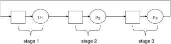
Figure 7.13: A three-stage closed queuing network.

(7.50) 

where N_i is the number of customers in the i queue. Also, since we have two customers:

(7.51) 

The state transition diagram for the system, with the states labeled as defined in equation (7.50), is shown in Figure 7.14. The labels on the edges denote customer movements from stage to stage and are dependent upon the service rate for the stage from which a customer is departing.

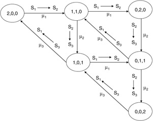
Figure 7.14: State transition rate diagram for a simple closed system.

To find the steady-state probabilities for each state in the system, we can write flow balance equations. As discussed earlier, the flow balance assumption states that we can represent the steady-state probabilities of a Markov process by writing the equations that balance the flow of customers into and out of the states in the network. For each individual state, then, we can write a balance equation that equates flow into a state with flow out of a state. For the states of Figure 7.14, we can write the following balance equations:

(7.52) 

(7.53) 

(7.54) 

(7.55) 

(7.56) 

(7.57) 

when:

• π(N₁, N₂, N₃) = Probability of state{N_l, N₂, N₃}

Keeping in mind that the sum of all of the state probabilities must equal 1, this network has the solution:

(7.58) 

where K is a normalization constant to ensure that the probabilities sum to 1:

(7.59)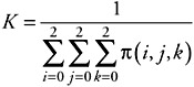 

Now, using equations 7.52 through 7.59, and the fact that all probabilities sum to 1, we can solve the flow balance equations for the individual state probabilities. Once we have the state probabilities, we can find the expected length at any of the servers, as follows:

(7.60)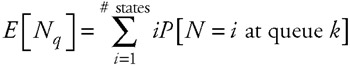 

Because the state probabilities at the queues are not the same as for the queuing systems in isolation, we cannot find the expected wait time in a queue by simply multiplying the number of customers by the service time at that queue. Instead, we will first calculate the throughput for each queuing system and then apply Little's result using the throughput as a measure of the arrival rate at a particular queue. Therefore, the throughput at a particular queue can be found by multiplying the probability of having a customer in that queue (e.g., the server is busy) times the expected service rate:

(7.61) 

Now, using Little's result, we can calculate the time spent in each queue by a customer at the respective queues:

(7.62) 

The total round-trip waiting time for a customer in the system can be found by summing up all of the queue waiting times. It can also be found directly by using Little's result and the average throughput for the system. Thus, for two customers, we have:

(7.63) 

Next, let's consider an arbitrary closed network with M queues and N customers. Assume that all servers have exponential service time distributions. For the sake of discussion, the network in Figure 7.15 will represent our arbitrary network. Let's define a branching probability as the probability of having any customer follow a particular branch when arriving at a branch point. Therefore, let:

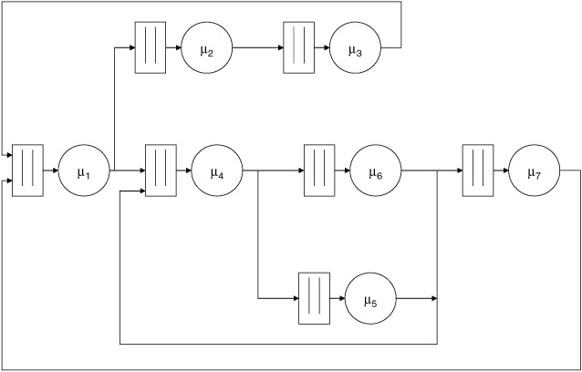
Figure 7.15: Arbitrary closed system.

(7.64) 

For any server i:

(7.65) 

The conservation of flow in the system requires that:

(7.66)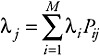 

Define the relative throughput of a server, i, as:

(7.67)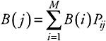 

Since the B terms are relative, we can arbitrarily set one of them equal to 1 and solve for the others. Once we have all of the terms, the steady-state probabilities are given by:

(7.68)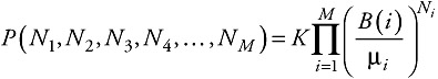 

Equation (7.67) can be derived by assuming the conservation of flow for a particular state and then by solving the system of equations as we did for the previous example. Let's pick a state, S, so that:

(7.69) 

and examine the effects of arrivals and departures of customers from queue j. Define another state, A, that is identical to S except that it has one more customer at queue i and one less customer at queue j than S. Thus, A is a neighbor state of S. We are postulating that the rate of entering state S due to an arrival at queue j is balanced by the rate of leaving state S due to a departure from queue j. Since there may be more than one state A, where there is one more customer at queue i and one less at j, we must balance all such states against state S. Equating the flows results in:

(7.70)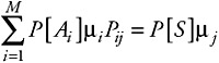 

From equation (7.68):

(7.71)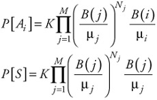 

The last term in each of the previous two expressions arises from having a customer in service at the respective servers. Substituting these expressions into equation (7.70) and simplifying, we get:

(7.72)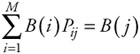 

which is what we postulated in equation (7.67).

Now that we have equation (7.72), we can generate a set of equations that we can solve simultaneously by setting one of the B terms equal to 1. In a manner similar to the previous example, we can also find the normalization constant K and therefore solve equation (7.68) for the system's steady-state probabilities and also for the expected queue lengths using equation (7.60).

If we consider the closed network over a long period of time, the relative throughput terms can be thought of as indicators of the relative number of times a customer visits the associated server, also called the visit ratio. This interpretation is useful for determining which server is the most utilized, also known as bottleneck analysis. Define the relative amount of work done by a server, i, as:

(7.73) 

Since this value is also the relative utilization of that server, the server with the highest such ratio is the system bottleneck.

7.2.2 Open networks

Next, we will discuss another class of queuing networks: those that contain sources and sinks. We will assume that customers may arrive at any queue from an outside source according to a Poisson process that is specific for that queue. We can think of these arrival processes as all originating from a single arrival process with branches, each with an associated branching probability. Figure 7.16 shows such an arrival process and a hypothetical open network with M queues and associated servers.

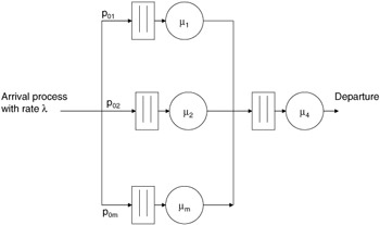
Figure 7.16: Open system model.

We also assume exponential service rates for all servers in the system. In this case, the aggregate arrival rate is equivalent to the sum of all of the individual arrival rates discussed earlier. If each individual arrival rate is defined as:

(7.74) 

the aggregate rate is given as:

(7.75) 

and the branching probabilities as:

(7.76) 

Customers leaving the system also do so with the probabilities defined as:

(7.77)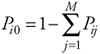 

This definition states that the probability of a job leaving the system is equal to the complement of the probability that a job will remain in the system.

As with the closed network discussed earlier, we can propose a set of throughput terms, denoted B(i) for each queue and server i. Thus:

(7.78)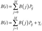 

Since we know the throughput arriving from the outside source, we can set:

(7.79) 

and solve for the remaining B terms. In the case of an open network, the B terms will represent actual, not relative, throughput at a server, i, because they are derived from the aggregate arrival rate. Because of this, we can define each server's utilization as:

(7.80) 

After solving for all of the B(i) terms, the steady-state probabilities are given as:

(7.81)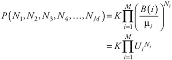 

where, again, K is a normalization constant. We can sum all of the state probabilities and solve for K to obtain:

(7.82)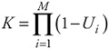 

Thus, the expression for the steady-state probabilities becomes:

(7.83)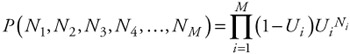 

If we look at equation (7.17), we see that the expression just derived is actually the product of terms that can be obtained by treating each queue and server as an M/M/1 queue system in isolation. This result is known as Jackson's theorem, and it states that, although the arrival rate at each server in an open system may not be Poisson, we can find the probability distribution function for the number of customers in any queue, as if the arrival process were Poisson (and, thereby, use equation [7.17] for the M/M/1 system). Jackson's theorem further states that each queue system in the network behaves as an M/M/1 system, with arrival rate defined by:

(7.84)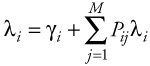 

which is simply equation (7.78) recast in more familiar terms.

It is worthwhile to note that Jackson's theorem applies to open systems in which the individual queue systems are M/M/C_i. That is, each server may actually be comprised of a different number (i) of identical servers. Thus, the steady-state probabilities for each queue system in the network are also given by the equation for such a system in isolation with the arrival rate, as described in equation (7.84). The full proof of Jackson's theorem is given in [8].

---