Finding Surface Normal Vectors
| | | ||||||||||||||||||||||||||
| ||||
| | ||||
Conic Sections and NURBS Curves
Conic sections are the family of curves that are generated when a plane intersects a cone. Depending on the angle between the cone and the plane, the resulting intersection can be elliptical , parabolic , or hyperbolic , as shown in Figure 5.8.
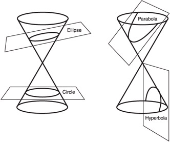
Figure 5.8: Conic Sections.
Most of the shapes shown in the previous chapters have been organic, free- flowing shapes. Organic shapes are useful, but it is also very useful to be able to draw shapes like circles (a special case of an ellipse). Unlike irrational B-splines, NURBS can be used to accurately represent conic sections.
Basic conic sections can be represented simply with quadratic (k=3) curves between three control points. The shape of the conic section is then determined by the relative weight of the middle control point. Figure 5.9 shows several different types of conic sections based on the same control points. The weight vector is [1 w 1].

Figure 5.9: Conic Sections from a quadratic curve.
When w is 0, a straight line is drawn between the first and last control points. When w is between 0 and 1, the resulting curve is elliptical. When w equals 1, the curve is parabolic. For all values greater than 1, the resulting curve is hyperbolic.
For the remainder of this chapter, I will concentrate on circles because they are probably the most common conic section you will use. Circular arcs are special cases of ellipses, so you know the value of w will be some value between 0 and 1.
To find that value, imagine the three control points defining an isosceles triangle that encloses the arc of a circle, as shown in Figure 5.10.

Figure 5.10: Defining an arc with an equilateral triangle.
From Figure 5.10, you can see that you need to pick a value of w such that the midpoint of the curve falls on the circle. Based on this, you can apply Equation 5.1 and a bit of geometry and trigonometry to find w as a function of the angle theta. After jumping through a few trigonometric hoops, you will find Equation 5.2.
| (5.2) w as a function of the angle of the arc. |  |
As Figure 5.11 shows, the simplest way to draw a circle is with three sets of arcs-120 degrees each. The final circle has a knot vector [X] = [0 0 0 1 1 2 2 3 3 3] and a weight vector [W] = [1.0 0.5 1.0 0.5 1.0 0.5 1.0]. These knot values result from Equation 5.2 applied to 120 degree arcs.

Figure 5.11: Defining a circle with a triangle.
A triangle might give you the simplest representation, but it gives you the fewest number of points to control. If you combine all the concepts seen so far, you can define the control points and weights in terms of the number of sides you want in the control polygon. This is demonstrated graphically in Figures 5.12 and 5.13.

Figure 5.12: Specifying circle controls in terms of the number of sides (N) of the control polygon.

Figure 5.13: Defining a square control polygon [X] = [0 0 0 1 1 2 2 3 3 4 4 4 ].
Once you can draw a circle, you can easily form an ellipse by moving the control points. You can also use a circle as a starting point for shapes that are symmetric about their center axis. Figure 5.14 shows how a circle can be used as a starting point for more interesting shapes.

Figure 5.14: Moving the control points of a circle.
Figures 5.11 and 5.13 are generated with the help of nonuniform knot vectors. Once you understand how to get the weighting factor for one of the segments, it is easy to see how to build a weight vector for several segments, but it may not be as easy to see how to build the concatenated knot vector. Remember that the knot vector defines the range of influence for each control point. With that in mind, I have supplied Figure 5.15 as a visual explanation of how a knot vector connects the individual arcs. Think of the knot values as quarters of the circle. The first two control points only influence the first quarter of the curve. The third and seventh control points affect the first and last half of the curve, respectively. If you have trouble figuring out what your knot vector should be, a diagram like Figure 5.15 can help.

Figure 5.15: Explaining the concatenated knot vector.
Once you understand how the knot vector (along with the order of the curve) affects the range of influence for each control point, it becomes very easy to generate curves that contain both conic sections and more organic shapes. Figure 5.16 shows such a curve. The last section of the curve is actually a quarter of a circle. I generated some random data for the first part of the curve, but I made sure to set the correct weight values, control point positions , and knot values for the circular section. The result is an erratic curve that ends with a smooth, mathematically correct circular arc.

Figure 5.16: Curve with conic section.
The most important point to take away from Figure 5.16 is the fact that curves do not need to be strictly defined as one type or another. There are several labels defined here (uniform, open , conic). These labels are useful for talking about certain properties of curves, but they should not necessarily be seen as constraints. Use the combinations of knots, weights, degrees, and control points that make the most sense for a given situation.
| | ||||
| ||||
| | ||||
EAN: 2147483647
Pages: 104