Using Classical Methods for Solving Equations
Problem
You've seen how to leverage Excel's built-in features to solve linear and nonlinear equations and systems, but you'd still like to know how to go about implementing some classical equation-solving algorithms in Excel.
Solution
You can use VBA to program any algorithm, just as you might in other programming languages. In the discussion to follow, I'll show you how to implement two classical methods in VBA: Newton's method and the secant method.
Discussion
The examples in this recipe will show how you might implement Newton's method and the secant method. These are well-known methods and are treated in most advanced mathematics and numerical methods texts. Further, you can find implementations of these methods in various languages, such as Fortran and C, on the Web. It's not a great leap to implement these methods in VBA in the form of a custom function, which you can then call from an Excel spreadsheet.
For the examples in this recipe, let's reconsider the cubic polynomial equation already discussed in Recipe 9.1. The equation is repeated here for convenience:

A quick plot of this equation, as shown earlier in Figure 9-6, shows about where these three roots lie. You could easily use Solver to accurately find each of these roots. Or, you could use Newton's method or the secant method (or any of a number of other methods you could program), as discussed in the remainder of this recipe.
Newton's method
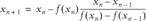
Newton's method is based on the idea of estimating values of x that are roots of the equation by taking the intersection of a line tangent to the curve under consideration at some assumed starting x-value. Subsequent estimates are made repeatedly using this approach until the estimate x-value converges on the true root. The basic formula for predicting each new x-value as you approach a root is:

Notice that in Newton's method you must be able to compute, or estimate, the first derivative of the curve under consideration. In the example considered here, we have an equation that allows you to explicitly compute the derivative. In other cases where you can't easily compute the derivative, or where it is impossible to do so explicitly (such as when part of your function relies on tabular data), you have to resort to numerical derivatives. Recall from the introduction to this chapter that Solver uses numerical derivatives and allows you to select either forward differencing or central differencing (refer to Recipe 10.6 for a discussion of these and other techniques).
The structure of the above equation should give you some hints as to how you might implement Newton's method. First, we need a subroutine to evaluate the function under consideration. Second, we need another subroutine to evaluate the derivative of that function. Third, we need a subroutine that will iteratively apply the above equation starting from some initial guess until it converges on a root. I've prepared just such subroutines for this example. The first one is shown in Example 9-5 and it is used to evaluate the function under consideration at some given x-value.
Example 9-5. Function Fx
Public Function Fx(x As Double) As Double Fx = 1 + x * (3 + x * (3 * x - 7)) End Function |
This subroutine is actually a Function, and therefore it returns a value to the calling subroutine. In this case, it returns the value of the cubic equation we're considering for this example. (If you were dealing with some other equation, you would change the function Fx accordingly.)
The next subroutine, shown in Example 9-6, is a Function that returns the derivative of our cubic equation for some given value of x.
Example 9-6. Function dFx
Public Function dFx(x As Double) As Double dFx = 3 + x * (9 * x - 14) End Function |
The final required subroutine is shown in Example 9-7 and actually implements Newton's method, making periodic calls to Fx and dFx.
Example 9-7. Newton's method
Public Function NewtonsMethod(x0 As Double, e As Double, n As Integer) As Double Dim i As Integer Dim err As Double Dim xn As Double Dim xn1 As Double i = 0 err = 9999 xn = x0 While (err > e) And (i < n) xn1 = xn - Fx(xn) / dFx(xn) err = Abs(xn1 - xn) xn = xn1 Wend NewtonsMethod = xn End Function |
Notice again that this subroutine, NewtonsMethod, is actually a Function. This means you'll be able to call it directly in a spreadsheet cell formula and it will return a result in the calling cell. I'll show you how shortly, but first I want to go through the function NewtonsMethod.
NewtonsMethod takes three parameters. The first one, x0, serves as your initial guess at a root. The second parameter, e, is a convergence tolerance, which should be a small real number (e.g., 0.001). e is used to determine when the function has converged on a possible root. The third and final parameter, n, is an iteration limit. It is used to prevent the function from iterating indefinitely in the event it can't converge on a root.
Several variables are declared upon entering the function. These include i, which is just a counter variable; err, which is used to store the difference between successive estimates for x; xn, which is used to store estimate xn; and xn1, which is used to store estimate xn+1.
Next, these variables are initialized. i is set to 0. err is set to some large number. And xn is set to the initial guess x0.
The While loop is where Newton's method is applied. The While loop will iterate until the computed error, err, is less than the convergence tolerance, e, or until the maximum number of iterations, n, has been reached.
A few things take place within the While loop. First, Newton's formula is applied, calling Fx and dFx to estimate the next x-value given the current estimate. Then the error is computed. Finally, the current x-estimate is updated before starting the next iteration.
When the While loop ends due either to converging on a root or reaching the iteration limit, the current estimate for x is returned by the function.
To call this function from a spreadsheet cell, you could enter something like =NewtonsMethod(0, 0.0001, 100) in any given cell. Excel will automatically call NewtonsMethod every time the spreadsheet needs updating (there's no need to use a button control, because NewtonsMethod is a Function). In this case, the cell will contain the value -0.215, which is indeed a root to the equation under consideration. Notice the initial guess I used here of 0.
To capture the other roots, you could change your initial guess. Changing the initial guess to 0.5 yields the root at x = 1.0. Again, changing the initial guess to 1.75 yields the root at x = 1.549.
Secant method
An alternative to Newton's method is the secant method . The secant method has the advantage that you do not need to compute the derivative of the equation under consideration. As a trade-off, you do have to supply two initial guesses so that a secant line can be constructed instead of a tangent line for making x predictions. The formula for estimating xn+1 using the secant method is:
To implement the secant method, we still need the function Fx as shown in Example 9-5, but we do not need the function dFx.
The VBA Function that implements the secant method for this example is shown in Example 9-8.
Example 9-8. Secant method
Public Function SecantMethod(x0 As Double, x1 As Double, e As Double, n As Integer) As Double Dim i As Integer Dim err As Double Dim xn As Double Dim xn1 As Double Dim xnm1 As Double i = 0 err = 9999 xn = x1 xnm1 = x0 While (err > e) And (i < n) xn1 = xn - Fx(xn) * (xn - xnm1) / (Fx(xn) - Fx(xnm1)) err = Abs(xn1 - xn) xnm1 = xn xn = xn1 Wend SecantMethod = xn End Function |
This function is substantially similar to the function NewtonsMethod. There are a few differences that I'll highlight. First, notice the additional parameter, x1, which represents the second initial guess for x. Remember that for the secant method we need two initial guesses for x.
The remaining differences are found within the While loop. As you can see, the expression for predicting xn1 has been replaced with the secant formula. And each iteration requires updating both xn and xn-1, which are stored in the variables xn and xnm1, respectively.
You can use SecantMethod in a cell formula just as you did NewtonsMethod. For example, I entered the following three formulas in three different cells in a spreadsheet:
 =secantmethod(0, -0.1, 0.0001, 100)
 =secantmethod(0.5, 0.6, 0.0001, 100)
 =secantmethod(1.75, 1.7, 0.0001, 100)
These three formulas returned the values -0.215, 1.000, and 1.549, respectively. As you see, these roots are identical to those obtained using Newton's method, and in both cases the results agree well with what you can glean by examining the plot of the example cubic equation in Figure 9-6.
Using Excel
- Introduction
- Navigating the Interface
- Entering Data
- Setting Cell Data Types
- Selecting More Than a Single Cell
- Entering Formulas
- Exploring the R1C1 Cell Reference Style
- Referring to More Than a Single Cell
- Understanding Operator Precedence
- Using Exponents in Formulas
- Exploring Functions
- Formatting Your Spreadsheets
- Defining Custom Format Styles
- Leveraging Copy, Cut, Paste, and Paste Special
- Using Cell Names (Like Programming Variables)
- Validating Data
- Taking Advantage of Macros
- Adding Comments and Equation Notes
- Getting Help
Getting Acquainted with Visual Basic for Applications
- Introduction
- Navigating the VBA Editor
- Writing Functions and Subroutines
- Working with Data Types
- Defining Variables
- Defining Constants
- Using Arrays
- Commenting Code
- Spanning Long Statements over Multiple Lines
- Using Conditional Statements
- Using Loops
- Debugging VBA Code
- Exploring VBAs Built-in Functions
- Exploring Excel Objects
- Creating Your Own Objects in VBA
- VBA Help
Collecting and Cleaning Up Data
- Introduction
- Importing Data from Text Files
- Importing Data from Delimited Text Files
- Importing Data Using Drag-and-Drop
- Importing Data from Access Databases
- Importing Data from Web Pages
- Parsing Data
- Removing Weird Characters from Imported Text
- Converting Units
- Sorting Data
- Filtering Data
- Looking Up Values in Tables
- Retrieving Data from XML Files
Charting
- Introduction
- Creating Simple Charts
- Exploring Chart Styles
- Formatting Charts
- Customizing Chart Axes
- Setting Log or Semilog Scales
- Using Multiple Axes
- Changing the Type of an Existing Chart
- Combining Chart Types
- Building 3D Surface Plots
- Preparing Contour Plots
- Annotating Charts
- Saving Custom Chart Types
- Copying Charts to Word
- Recipe 4-14. Displaying Error Bars
Statistical Analysis
- Introduction
- Computing Summary Statistics
- Plotting Frequency Distributions
- Calculating Confidence Intervals
- Correlating Data
- Ranking and Percentiles
- Performing Statistical Tests
- Conducting ANOVA
- Generating Random Numbers
- Sampling Data
Time Series Analysis
- Introduction
- Plotting Time Series Data
- Adding Trendlines
- Computing Moving Averages
- Smoothing Data Using Weighted Averages
- Centering Data
- Detrending a Time Series
- Estimating Seasonal Indices
- Deseasonalization of a Time Series
- Forecasting
- Applying Discrete Fourier Transforms
Mathematical Functions
- Introduction
- Using Summation Functions
- Delving into Division
- Mastering Multiplication
- Exploring Exponential and Logarithmic Functions
- Using Trigonometry Functions
- Seeing Signs
- Getting to the Root of Things
- Rounding and Truncating Numbers
- Converting Between Number Systems
- Manipulating Matrices
- Building Support for Vectors
- Using Spreadsheet Functions in VBA Code
- Dealing with Complex Numbers
Curve Fitting and Regression
- Introduction
- Performing Linear Curve Fitting Using Excel Charts
- Constructing Your Own Linear Fit Using Spreadsheet Functions
- Using a Single Spreadsheet Function for Linear Curve Fitting
- Performing Multiple Linear Regression
- Generating Nonlinear Curve Fits Using Excel Charts
- Fitting Nonlinear Curves Using Solver
- Assessing Goodness of Fit
- Computing Confidence Intervals
Solving Equations
- Introduction
- Finding Roots Graphically
- Solving Nonlinear Equations Iteratively
- Automating Tedious Problems with VBA
- Solving Linear Systems
- Tackling Nonlinear Systems of Equations
- Using Classical Methods for Solving Equations
Numerical Integration and Differentiation
- Introduction
- Integrating a Definite Integral
- Implementing the Trapezoidal Rule in VBA
- Computing the Center of an Area Using Numerical Integration
- Calculating the Second Moment of an Area
- Dealing with Double Integrals
- Numerical Differentiation
Solving Ordinary Differential Equations
- Introduction
- Solving First-Order Initial Value Problems
- Applying the Runge-Kutta Method to Second-Order Initial Value Problems
- Tackling Coupled Equations
- Shooting Boundary Value Problems
Solving Partial Differential Equations
- Introduction
- Leveraging Excel to Directly Solve Finite Difference Equations
- Recruiting Solver to Iteratively Solve Finite Difference Equations
- Solving Initial Value Problems
- Using Excel to Help Solve Problems Formulated Using the Finite Element Method
Performing Optimization Analyses in Excel
- Introduction
- Using Excel for Traditional Linear Programming
- Exploring Resource Allocation Optimization Problems
- Getting More Realistic Results with Integer Constraints
- Tackling Troublesome Problems
- Optimizing Engineering Design Problems
- Understanding Solver Reports
- Programming a Genetic Algorithm for Optimization
Introduction to Financial Calculations
- Introduction
- Computing Present Value
- Calculating Future Value
- Figuring Out Required Rate of Return
- Doubling Your Money
- Determining Monthly Payments
- Considering Cash Flow Alternatives
- Achieving a Certain Future Value
- Assessing Net Present Worth
- Estimating Rate of Return
- Solving Inverse Problems
- Figuring a Break-Even Point
Index
EAN: 2147483647
Pages: 206
