OEM and Tuning
| In previous chapters, you have seen how the Oracle Enterprise Manager (OEM) has helped administrators and developers obtain quick insights into and help manage the database via an easy-to-use graphical user interface. This section will show how OEM can help the performance analyst view and interpret performance statistics. Simply stated, OEM is packaged in two forms:
The main difference between these as far as this section is concerned is in the login process. Assuming that both components are installed and configured, in order to manage a single database via Database Control, you would log in directly to the database using the correct URL. If you wanted to manage a single database that has been configured as part of a Grid Control environment, you would first log in to the OEM Grid Control console using the correct URL, and then choose the required targetin this case, a database. When this is complete, all actions are the same. Hence, for the purpose of this section, we will assume that you are logging into the TS10G database on a host named test10g using the Database Control via the following URL: http://test10g:5550/em.
This will bring up a login page, where you will first log in using the SYS or SYSTEM account. When this is done, depending on your requirement, you can create additional Database Control users that can be used by a designated set of other personnel. We will concern ourselves only with the performance menus and functions at this time. There are numerous pages, menus, submenus, area graphs, drill-downs, and hyperlinks available for performance monitoring and reporting. Rather than detail all of them, we will highlight those that are most useful. Navigating OEM Database ControlIn OEM Database Control, you can get to the same information using a variety of paths. For example, you can get to the Top Sessions detail page via either of the following routes:
General Database and Host InformationAnalyzing database performance without considering the underlying operating system will result in both an incomplete and incorrect diagnosis. OEM in Oracle Database 10g provides lots of information about the database as well as the host operating system, as compared to earlier versions. Host information includes CPU statistics categorized by both database and other types of processes, CPU utilization, CPU I/O wait, CPU load, run queue length, paging rate, and so on, as well as session information such as CPU, I/O, and categorized waits. An incredible amount of drill-down information is available at all levels in both tabular and graphical form. These drill-downs are contextual and appropriate, providing for in-depth analysis without unnecessary clutter. Graphs include line and stacked charts for representing values against time scales, and pie charts when representing percentages of an entity. Most screens refresh themselves in real time and can thus impose an unnecessary load on the system. On a heavily loaded system, use the Interval drop-down menu to change the rate to Manual. When historical information is available, choosing this option brings up options to view successively larger intervals, usually for the past 24 hours, past seven days, and so on. The highlight, however, is the availability of a slider tool in many screens that can be used to drag a shaded box over to the selected interval.
A Quick ExampleThis section demonstrates the use of OEM Database Control for performance diagnosis and tuning quickly using a very simple example. We will use a few objects from the HR schema from the sample schemas that are shipped along with the Oracle Database 10g and are installed by the DBCA installation assistant. For further details, refer to the Oracle Database 10g Sample Schema manual. The example shown here is a simple way of generating an enormous but controlled load on the system. You will notice that we used very simple techniques and tools already available in the UNIX operating system command-line commands. It could very well be generated using Windows command scripts with the FOR statement. We used the SQL shown in Listing 10.12 to create a large number of rows in the EMPLOYEES table of the HR schema. No extra objects need to be created, although the widths of the FIRST_NAME, LAST_NAME, and EMAIL columns were increased to an even VARCHAR2(50) from their default. Listing 10.12. Script to Generate a Large Number of Rows in the EMPLOYEES Tableinsert into employees ( employee_id, first_name, last_name, email, phone_number, hire_date, job_id, salary, commission_pct, manager_id, department_id ) select employees_seq.nextval , first_name || ' ' || employees_seq.currval , last_name|| ' ' || employees_seq.currval , email|| ' ' || employees_seq.currval , phone_number, hire_date , job_id, salary, commission_pct, manager_id, department_id from employees; This SQL copies the current set of rows in the EMPLOYEES table into itself, while generating new key values for the EMPLOYEE_ID as well as concatenating new numeric values to the employee details. This generates a fairly even spread of rows, each distinct from the others in some way. Executing this SQL a number of times will successively insert a larger and larger number of rows. For example, the first time this SQL is run in the HR schema, it doubles the 107 rows. Running this SQL again will double the result, with a final total of (107 + 107 + 314 = 628) rows. Run the SQL as many times as requiredwe tested this out with 14,000 rows in the EMPLOYEES table. We then used the following embedded query to extract the employee data held in the sample HR schema. To complicate the SQL and provide many type of joins and opportunities for tuning, we joined the detail table, namely EMPLOYEES, to the other master tables such as REGIONS, DEPARTMENTS, LOCATIONS, and COUNTRIES as shown in the SQL statement in Listing 10.13. The following UNIX shell script segment was then used to generate a large but set number of executions by wrapping the SQL in a shell script named multi.ksh, shown in Listing 10.13. Listing 10.13. UNIX Script for Simulating a Large User Loadi=1 while [ $i -le 100 ] # Control number of executions using this number do echo $i sqlplus -silent hr/hr123 <<EOF > $i.out 2>&1 & # Use the & to launch in the background set termout off select e.* from hr.employees e, hr.departments d, hr.locations l, hr.countries c, hr.regions r where e.department_id = d.department_id and d.location_id = l.location_id and l.country_id = c.country_id and c.region_id = r.region_id and employee_id between substr(to_char(abs(dbms_random.random)),1,4) and substr(to_char(abs(dbms_random.random)),1,4); exit EOF sleep 1 # Sleep for a brief second i=`expr $i + 1` done wait # Wait after launching a number of SQLs in the background echo All done! The call DBMS_RANDOM.RANDOM generates a random number. You apply some transformations to obtain a starting and ending number, each of which could range from 0 to 9,999. When the first random number is larger than the second, no rows were selected, so some of the SQLs do not return any rows. On the other hand, some of the other SQLs select a lot of rows, all at random. This simply and perfectly simulates a live system with random queries and load. Main OEM Performance-Related ScreensAfter the test started, we logged on to the Enterprise Manager Database Console using the SYSTEM account. You can also use another user with access to the Database Control to view the results. Snapshots of relevant portions are shown in subsequent paragraphs with explanations. The Database Control home page is displayed upon successful login to OEM Database Control, as shown in Figure 10.1. This screen displays quite a handful of information, including the overall system health for all areas. We will zoom in only on the relevant areas, namely the graphs that show the operating system as well as the Session area. Figure 10.1. The OEM Database Control home page showing relevant performance areas.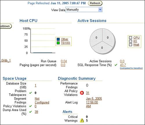 When you click on the Wait link in the Session area, you will see the host and session information relevant to waiting, as shown in Figure 10.2. This shows the overall performance for the host, session, and throughput in real time. You can switch this to Historical view or to a Manual refresh view to enable going back to or stopping the screen for further drill-downs. Notice the line across Maximum CPU; we had two CPUs in this case. Figure 10.2. Performance page showing host and database wait information.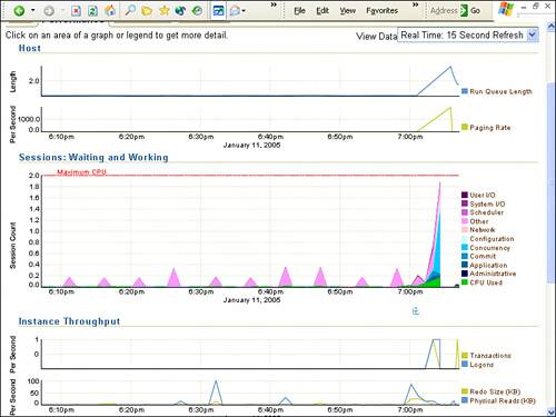 Session waits are classified into many categories, such as User I/O and System I/O, Concurrency, Application, and so on. You can link this directly to the Wait class categories seen earlier. The host run queue length, which is a measure of "waiting for CPU" is also seen on this Wait page. This helps you appreciate how the designers of OEM have kept the related details together so a performance analyst can see both database and operating-system statistics together, helping to determine root causes and the relationships quickly and intuitively. When you hover the cursor over the Concurrency section of the Sessions: Waiting and Working graph shown in Figure 10.2, the Concurrency portion of the graph is highlighted. As well, you can click and drill down to get the reasons for the concurrency issue for the selected period. This drill-down screen, shown in Figure 10.3, shows the waits related specifically to the Concurrency wait class. As mentioned previously, this can relate to latching or internal concurrency as well as to row or other resource locking, which is external concurrency. Figure 10.3. Page showing concurrency-related wait information.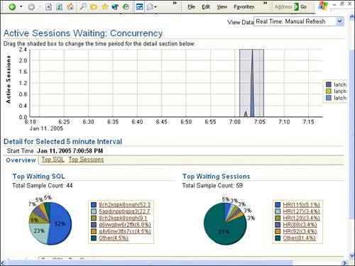 This is a historical view; hence, we were able to drag the slider tool over to the time period of interest. This slider is shown with a darkened background, and can be set to a period of as little as five minutes and as large as a day. Note that we have not drilled down into all the subsections in this page. You can determine Top SQL as well as Top Sessions in the lower part of the screen. You can see that there were about three active concurrent sessions out of 59 connected sessions, and that the SQL run by at least one of them contributed to 52% of the waits. Specifically, this was broken down into latch: session allocation and latch free (not shown in the figure due to screen-shot limitations). You can now drill down into the details of the top SQL statements that contributed to the majority of the waits. In this specific case, drill down into the SQL using the links shown against the SQL hash values. In particular, the screen shown in Figure 10.4 is displayed when you click on the top-most link that corresponds to the SQL statement emanating from the shell script shown in Listing 10.13. Figure 10.4. Details of the Top SQL, which contributed to 52% of the waits.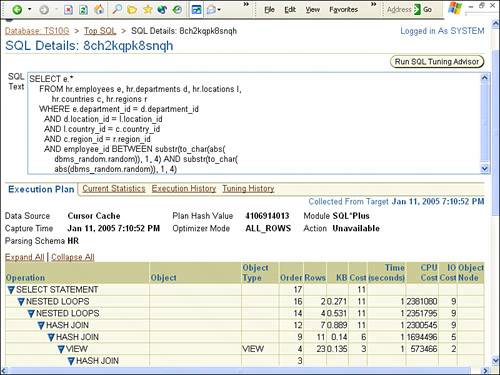 Figure 10.4 shows the SQL that contributed most to the waiting. As expected, it was the SQL that was executed simultaneously from many sessions. The SQL is shown along with the execution plan and other parameters. Because this was a Top SQL and is possibly worth tuning, OEM provides an easy link to the aptly named SQL Tuning Advisor, shown in Figure 10.5, via the Run SQL Tuning Advisor button. Figure 10.5. SQL Tuning Advisor scheduling screen.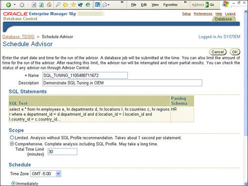 The SQL Tuning Advisor can apply various tuning scenarios on the selected SQL and needs some scheduling parameters, as seen in Figure 10.5. Choosing the required parameters and allowing the advisor to operate results in the screen shown in Figure 10.6. Figure 10.6. SQL Tuning Advisor results, showing recommendations.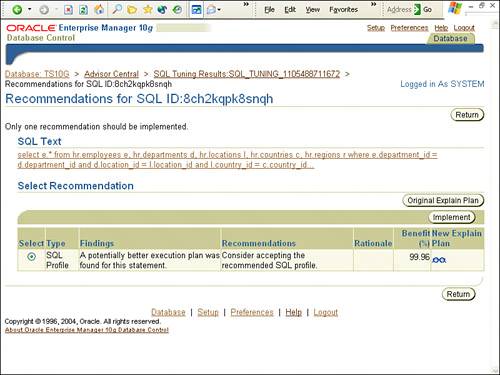 As you can see, SQL Tuning Advisor recommends that this SQL be tuned using an SQL profile. We will look at this type of tuning in depth in Chapter 13, "Effectively Using the SQL Advisors," so we will not go into details now. In any case, you might want to view the changed execution plan before accepting it. To do so, click on the eyeglasses shown in Figure 10.6. This will result in the tuned execution plan for the same SQL, as shown in Figure 10.7. Figure 10.7. Details of the new explain plan.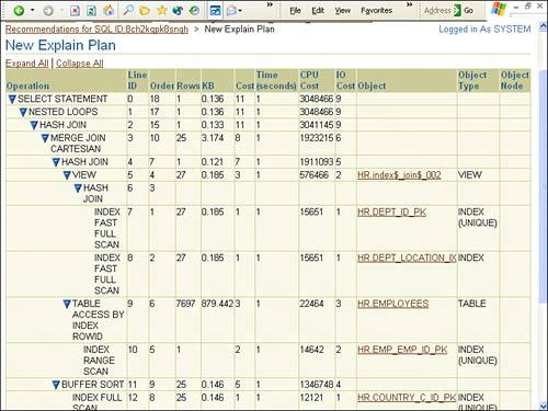 You can then compare this to the older execution plan, as shown in Figure 10.8, by clicking the Original Explain Plan button in Figure 10.6. Figure 10.8. Details of the original explain plan.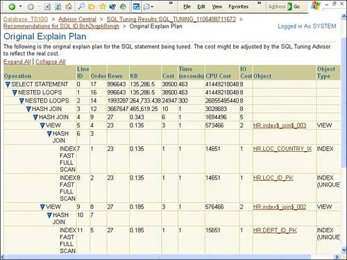 That is not all. Shown in Figure 10.9 are some other statistics obtained from the OEM Database Control. To access these, from the home page, click on the Other link in the Host graph. Figure 10.9. Host performance summary showing CPU, memory, and disk I/O utilization.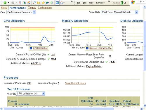 Notice the View drop-down menu at the top-left side of the screen. This shows the Performance Summary option by default, which includes utilization graphs for CPU, memory, and disk I/O. By default, the lower portion of the screen displays top processes by CPU consumption as well. This section can be changed via the View Data drop-down menu, found in the top-right corner of the screen. Use this menu to control the rate of refresh or to view the history for this statistic. You can drill down further by choosing CPU Details or Memory Details from the View drop-down menu. This results in the screens displayed in Figure 10.10 for CPU details and Figure 10.11 for memory details. Figure 10.10. Host performance CPU drill-down details as well as top CPU processes.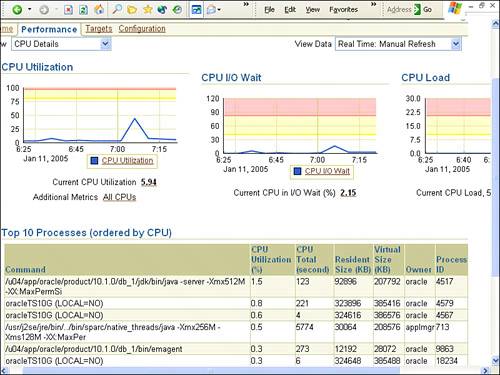 Figure 10.11. Host performance Memory drill-down details as well as top memory processes.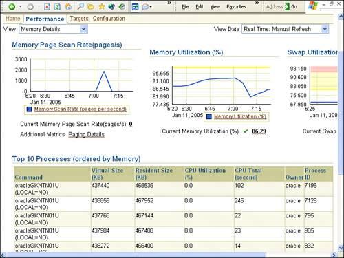 Note that the bottom part of the screen automatically varies between the two figures, first to display the Top 10 Processes (ordered by CPU) and then to display the Top 10 Processes (ordered by Memory), keeping in sync with the type of statistics displayed above. Alerts and MetricsNot everything is displayed via graphs in OEM. A good example is the Metrics screen, which you access by clicking the All Metrics link that is available on all pages. A sample Metrics page is shown in Figure 10.12. Figure 10.12. The All Metrics page.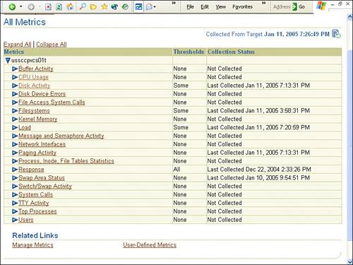 A large number of alerts, including performance alerts, are configured out of the box in OEM. These are available as links in the bottom of most pages. These screens display all alerts, including performance alerts such as Database Time spent Waiting. Use the Manage Metrics link on this page to view the details of these metrics and the Edit Thresholds button to enable/disable alerts and to change the various thresholds for the Warning and Critical levels. You can also specify response actions, which are triggered when these alerts are triggered, as well as multiple thresholds at which they trigger. This is a very powerful option that is sure to replace many other third-party and home-grown tools and scripts. AdvisorsNumerous advisors can be accessed via the Advisor Central link in the Related Links section in most pages. They include the following:
We will look in greater detail at some of these advisors in later chapters. |
EAN: 2147483647
Pages: 214